Introduction
The Open Shortest Path First (OSPF) protocol, defined in RFC 2328, is an Interior Gateway Protocol used to distribute routing information within a single Autonomous System. This paper examines how OSPF works and how it can be used to design and build large and complicated networks.Background Information
OSPF protocol was developed due to a need in the internet community to introduce a high functionality non-proprietary Internal Gateway Protocol (IGP) for the TCP/IP protocol family. The discussion of the creation of a common interoperable IGP for the Internet started in 1988 and did not get formalized until 1991. At that time the OSPF Working Group requested that OSPF be considered for advancement to Draft Internet Standard.The OSPF protocol is based on link-state technology, which is a departure from the Bellman-Ford vector based algorithms used in traditional Internet routing protocols such as RIP. OSPF has introduced new concepts such as authentication of routing updates, Variable Length Subnet Masks (VLSM), route summarization, and so forth.
These chapters discuss the OSPF terminology, algorithm and the pros and cons of the protocol in designing the large and complicated networks of today.
OSPF versus RIP
The rapid growth and expansion of today's networks has pushed RIP to its limits. RIP has certain limitations that can cause problems in large networks:-
RIP has a limit of 15 hops. A RIP network that spans more than 15
hops (15 routers) is considered unreachable.
-
RIP cannot handle Variable Length Subnet Masks (VLSM). Given the
shortage of IP addresses and the flexibility VLSM gives in the efficient
assignment of IP addresses, this is considered a major flaw.
-
Periodic broadcasts of the full routing table consume a large amount
of bandwidth. This is a major problem with large networks especially on slow
links and WAN clouds.
-
RIP converges slower than OSPF. In large networks convergence gets to
be in the order of minutes. RIP routers go through a period of a hold-down and
garbage collection and slowly time-out information that has not been received
recently. This is inappropriate in large environments and could cause routing
inconsistencies.
-
RIP has no concept of network delays and link costs. Routing
decisions are based on hop counts. The path with the lowest hop count to the
destination is always preferred even if the longer path has a better aggregate
link bandwidth and less delays.
-
RIP networks are flat networks. There is no concept of areas or
boundaries. With the introduction of classless routing and the intelligent use
of aggregation and summarization, RIP networks seem to have fallen behind.
OSPF, on the other hand, addresses most of the issues previously presented:
-
With OSPF, there is no limitation on the hop count.
-
The intelligent use of VLSM is very useful in IP address
allocation.
-
OSPF uses IP multicast to send link-state updates. This ensures less
processing on routers that are not listening to OSPF packets. Also, updates are
only sent in case routing changes occur instead of periodically. This ensures a
better use of bandwidth.
-
OSPF has better convergence than RIP. This is because routing changes
are propagated instantaneously and not periodically.
-
OSPF allows for better load balancing.
-
OSPF allows for a logical definition of networks where routers can be
divided into areas. This limits the explosion of link state updates over the
whole network. This also provides a mechanism for aggregating routes and
cutting down on the unnecessary propagation of subnet
information.
-
OSPF allows for routing authentication by using different methods of
password authentication.
-
OSPF allows for the transfer and tagging of external routes injected
into an Autonomous System. This keeps track of external routes injected by
exterior protocols such as BGP.
What Do We Mean by Link-States?
OSPF is a link-state protocol. We could think of a link as being an interface on the router. The state of the link is a description of that interface and of its relationship to its neighboring routers. A description of the interface would include, for example, the IP address of the interface, the mask, the type of network it is connected to, the routers connected to that network and so on. The collection of all these link-states would form a link-state database.Shortest Path First Algorithm
OSPF uses a shorted path first algorithm in order to build and calculate the shortest path to all known destinations.The shortest path is calculated with the use of the Dijkstra algorithm. The algorithm by itself is quite complicated. This is a very high level, simplified way of looking at the various steps of the algorithm:-
Upon initialization or due to any change in routing information, a
router generates a link-state advertisement. This advertisement represents the
collection of all link-states on that router.
-
All routers exchange link-states by means of flooding. Each router
that receives a link-state update should store a copy in its link-state
database and then propagate the update to other routers.
-
After the database of each router is completed, the router calculates
a Shortest Path Tree to all destinations. The router uses the Dijkstra
algorithm in order to calculate the shortest path tree. The destinations, the
associated cost and the next hop to reach those destinations form the IP
routing table.
-
In case no changes in the OSPF network occur, such as cost of a link
or a network being added or deleted, OSPF should be very quiet. Any changes
that occur are communicated through link-state packets, and the Dijkstra
algorithm is recalculated in order to find the shortest path.
OSPF Cost
The cost (also called metric) of an interface in OSPF is an indication of the overhead required to send packets across a certain interface. The cost of an interface is inversely proportional to the bandwidth of that interface. A higher bandwidth indicates a lower cost. There is more overhead (higher cost) and time delays involved in crossing a 56k serial line than crossing a 10M ethernet line. The formula used to calculate the cost is:-
cost= 10000 0000/bandwith in bps
By default, the cost of an interface is calculated based on the bandwidth; you can force the cost of an interface with the ip ospf cost
Shortest Path Tree
Assume we have the following network diagram with the indicated interface costs. In order to build the shortest path tree for RTA, we would have to make RTA the root of the tree and calculate the smallest cost for each destination.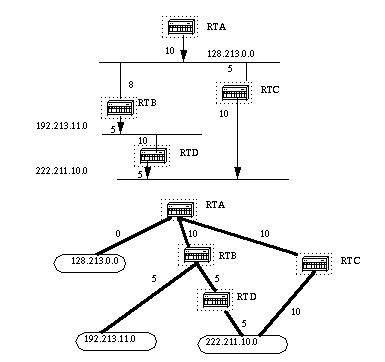
The above is the view of the network as seen from RTA. Note the direction of the arrows in calculating the cost. For example, the cost of RTB's interface to network 128.213.0.0 is not relevant when calculating the cost to 192.213.11.0. RTA can reach 192.213.11.0 via RTB with a cost of 15 (10+5). RTA can also reach 222.211.10.0 via RTC with a cost of 20 (10+10) or via RTB with a cost of 20 (10+5+5). In case equal cost paths exist to the same destination, Cisco's implementation of OSPF will keep track of up to six next hops to the same destination.
After the router builds the shortest path tree, it will start building the routing table accordingly. Directly connected networks will be reached via a metric (cost) of 0 and other networks will be reached according to the cost calculated in the tree.
Areas and Border Routers
As previously mentioned, OSPF uses flooding to exchange link-state updates between routers. Any change in routing information is flooded to all routers in the network. Areas are introduced to put a boundary on the explosion of link-state updates. Flooding and calculation of the Dijkstra algorithm on a router is limited to changes within an area. All routers within an area have the exact link-state database. Routers that belong to multiple areas, and connect these areas to the backbone area are called area border routers (ABR). ABRs must therefore maintain information describing the backbone areas and other attached areas.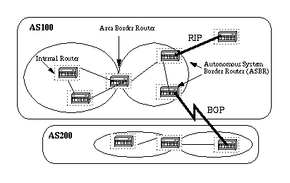
An area is interface specific. A router that has all of its interfaces within the same area is called an internal router (IR). A router that has interfaces in multiple areas is called an area border router (ABR). Routers that act as gateways (redistribution)between OSPF and other routing protocols (IGRP, EIGRP, IS-IS, RIP, BGP, Static) or other instances of the OSPF routing process are called autonomous system boundary router (ASBR). Any router can be an ABR or an ASBR.
Link-State Packets
There are different types of Link State Packets, those are what you normally see in an OSPF database (Appendix A). The different types are illustrated in the following diagram: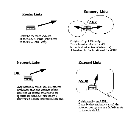
As indicated above, the router links are an indication of the state of the interfaces on a router belonging to a certain area. Each router will generate a router link for all of its interfaces. Summary links are generated by ABRs; this is how network reachability information is disseminated between areas. Normally, all information is injected into the backbone (area 0) and in turn the backbone will pass it on to other areas. ABRs also have the task of propagating the reachability of the ASBR. This is how routers know how to get to external routes in other ASs.
Network Links are generated by a Designated Router (DR) on a segment (DRs will be discussed later). This information is an indication of all routers connected to a particular multi-access segment such as Ethernet, Token Ring and FDDI (NBMA also).
External Links are an indication of networks outside of the AS. These networks are injected into OSPF via redistribution. The ASBR has the task of injecting these routes into an autonomous system.
Enabling OSPF on the Router
Enabling OSPF on the router involves the following two steps in config mode:-
Enabling an OSPF process using the router ospf
command.
-
Assigning areas to the interfaces using the network
The network command is a way of assigning an interface to a certain area. The mask is used as a shortcut and it helps putting a list of interfaces in the same area with one line configuration line. The mask contains wild card bits where 0 is a match and 1 is a "do not care" bit, e.g. 0.0.255.255 indicates a match in the first two bytes of the network number.
The area-id is the area number we want the interface to be in. The area-id can be an integer between 0 and 4294967295 or can take a form similar to an IP address A.B.C.D.
Here's an example:
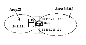
The first network statement puts both E0 and E1 in the same area 0.0.0.0, and the second network statement puts E2 in area 23. Note the mask of 0.0.0.0, which indicates a full match on the IP address. This is an easy way to put an interface in a certain area if you are having problems figuring out a mask.RTA# interface Ethernet0 ip address 192.213.11.1 255.255.255.0 interface Ethernet1 ip address 192.213.12.2 255.255.255.0 interface Ethernet2 ip address 128.213.1.1 255.255.255.0 router ospf 100 network 192.213.0.0 0.0.255.255 area 0.0.0.0 network 128.213.1.1 0.0.0.0 area 23
OSPF Authentication
It is possible to authenticate the OSPF packets such that routers can participate in routing domains based on predefined passwords. By default, a router uses a Null authentication which means that routing exchanges over a network are not authenticated. Two other authentication methods exist: Simple password authentication and Message Digest authentication (MD-5).Simple Password Authentication
Simple password authentication allows a password (key) to be configured per area. Routers in the same area that want to participate in the routing domain will have to be configured with the same key. The drawback of this method is that it is vulnerable to passive attacks. Anybody with a link analyzer could easily get the password off the wire. To enable password authentication use the following commands:-
ip
ospf authentication-key key (this
goes under the specific interface)
-
area area-id authentication (this goes
under "router ospf
")
interface Ethernet0
ip address 10.10.10.10 255.255.255.0
ip ospf authentication-key mypassword

router ospf 10
network 10.10.0.0 0.0.255.255 area 0
area 0 authentication
Message Digest Authentication
Message Digest authentication is a cryptographic authentication. A key (password) and key-id are configured on each router. The router uses an algorithm based on the OSPF packet, the key, and the key-id to generate a "message digest" that gets appended to the packet. Unlike the simple authentication, the key is not exchanged over the wire. A non-decreasing sequence number is also included in each OSPF packet to protect against replay attacks.This method also allows for uninterrupted transitions between keys. This is helpful for administrators who wish to change the OSPF password without disrupting communication. If an interface is configured with a new key, the router will send multiple copies of the same packet, each authenticated by different keys. The router will stop sending duplicate packets once it detects that all of its neighbors have adopted the new key. Following are the commands used for message digest authentication:
-
ip
ospf message-digest-key keyid md5 key (used under the interface)
-
area area-id authentication
message-digest (used under "router ospf
")
interface Ethernet0
ip address 10.10.10.10 255.255.255.0
ip ospf message-digest-key 10 md5 mypassword

router ospf 10
network 10.10.0.0 0.0.255.255 area 0
area 0 authentication message-digest
The Backbone and Area 0
OSPF has special restrictions when multiple areas are involved. If more than one area is configured, one of these areas has be to be area 0. This is called the backbone. When designing networks it is good practice to start with area 0 and then expand into other areas later on.The backbone has to be at the center of all other areas, i.e. all areas have to be physically connected to the backbone. The reasoning behind this is that OSPF expects all areas to inject routing information into the backbone and in turn the backbone will disseminate that information into other areas. The following diagram will illustrate the flow of information in an OSPF network:
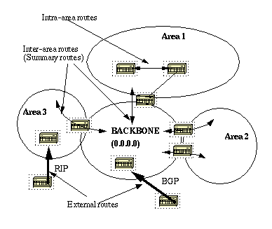
In the above diagram, all areas are directly connected to the backbone. In the rare situations where a new area is introduced that cannot have a direct physical access to the backbone, a virtual link will have to be configured. Virtual links will be discussed in the next section. Note the different types of routing information. Routes that are generated from within an area (the destination belongs to the area) are called intra-area routes. These routes are normally represented by the letter O in the IP routing table. Routes that originate from other areas are called inter-area or Summary routes. The notation for these routes is O IA in the IP routing table. Routes that originate from other routing protocols (or different OSPF processes) and that are injected into OSPF via redistribution are called external routes. These routes are represented by O E2 or O E1 in the IP routing table. Multiple routes to the same destination are preferred in the following order: intra-area, inter-area, external E1, external E2. External types E1 and E2 will be explained later.
Virtual Links
Virtual links are used for two purposes:-
Linking an area that does not have a physical connection to the
backbone.
-
Patching the backbone in case discontinuity of area 0 occurs.
Areas Not Physically Connected to Area 0
As mentioned earlier, area 0 has to be at the center of all other areas. In some rare case where it is impossible to have an area physically connected to the backbone, a virtual link is used. The virtual link will provide the disconnected area a logical path to the backbone. The virtual link has to be established between two ABRs that have a common area, with one ABR connected to the backbone. This is illustrated in the following example: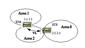
In this example, area 1 does not have a direct physical connection into area 0. A virtual link has to be configured between RTA and RTB. Area 2 is to be used as a transit area and RTB is the entry point into area 0. This way RTA and area 1 will have a logical connection to the backbone. In order to configure a virtual link, use the area
RTA#
router ospf 10
area 2 virtual-link 2.2.2.2


RTB#
router ospf 10
area 2 virtual-link 1.1.1.1
Partitioning the Backbone
OSPF allows for linking discontinuous parts of the backbone using a virtual link. In some cases, different area 0s need to be linked together. This can occur if, for example, a company is trying to merge two separate OSPF networks into one network with a common area 0. In other instances, virtual-links are added for redundancy in case some router failure causes the backbone to be split into two. Whatever the reason may be, a virtual link can be configured between separate ABRs that touch area 0 from each side and having a common area. This is illustrated in the following example: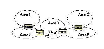
In the above diagram two area 0s are linked together via a virtual link. In case a common area does not exist, an additional area, such as area 3, could be created to become the transit area.
In case any area which is different than the backbone becomes partitioned, the backbone will take care of the partitioning without using any virtual links. One part of the partioned area will be known to the other part via inter-area routes rather than intra-area routes.
Neighbors
Routers that share a common segment become neighbors on that segment. Neighbors are elected via the Hello protocol. Hello packets are sent periodically out of each interface using IP multicast (Appendix B). Routers become neighbors as soon as they see themselves listed in the neighbor's Hello packet. This way, a two way communication is guaranteed. Neighbor negotiation applies to the primary address only. Secondary addresses can be configured on an interface with a restriction that they have to belong to the same area as the primary address.Two routers will not become neighbors unless they agree on the following:
-
Area-id: Two routers having a common segment; their
interfaces have to belong to the same area on that segment. Of course, the
interfaces should belong to the same subnet and have a similar mask.
-
Authentication: OSPF allows for the configuration of
a password for a specific area. Routers that want to become neighbors have to
exchange the same password on a particular segment.
-
Hello and Dead Intervals: OSPF exchanges Hello
packets on each segment. This is a form of keepalive used by routers in order
to acknowledge their existence on a segment and in order to elect a designated
router (DR) on multiaccess segments.The Hello interval specifies the length of
time, in seconds, between the hello packets that a router sends on an OSPF
interface. The dead interval is the number of seconds that a router's Hello
packets have not been seen before its neighbors declare the OSPF router down.
OSPF requires these intervals to be exactly the same between two neighbors. If any of these intervals are different, these routers will not become neighbors on a particular segment. The router interface commands used to set these timers are: ip ospf hello-interval seconds and ip ospf dead-interval seconds .
-
Stub area flag: Two routers have to also agree on
the stub area flag in the Hello packets in order to become neighbors. Stub
areas will be discussed in a later section. Keep in mind for now that defining
stub areas will affect the neighbor election process.
Adjacencies
Adjacency is the next step after the neighboring process. Adjacent routers are routers that go beyond the simple Hello exchange and proceed into the database exchange process. In order to minimize the amount of information exchange on a particular segment, OSPF elects one router to be a designated router (DR), and one router to be a backup designated router (BDR), on each multi-access segment. The BDR is elected as a backup mechanism in case the DR goes down. The idea behind this is that routers have a central point of contact for information exchange. Instead of each router exchanging updates with every other router on the segment, every router exchanges information with the DR and BDR. The DR and BDR relay the information to everybody else. In mathematical terms, this cuts the information exchange from O(n*n) to O(n) where n is the number of routers on a multi-access segment. The following router model illustrates the DR and BDR: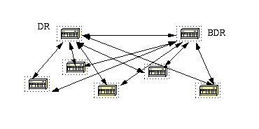
In the above diagram, all routers share a common multi-access segment. Due to the exchange of Hello packets, one router is elected DR and another is elected BDR. Each router on the segment (which already became a neighbor) will try to establish an adjacency with the DR and BDR.
DR Election
DR and BDR election is done via the Hello protocol. Hello packets are exchanged via IP multicast packets (Appendix B) on each segment. The router with the highest OSPF priority on a segment will become the DR for that segment. The same process is repeated for the BDR. In case of a tie, the router with the highest RID will win. The default for the interface OSPF priority is one. Remember that the DR and BDR concepts are per multiaccess segment. Setting the ospf priority on an interface is done using the ip ospf priorityA priority value of zero indicates an interface which is not to be elected as DR or BDR. The state of the interface with priority zero will be DROTHER. The following diagram illustrates the DR election:
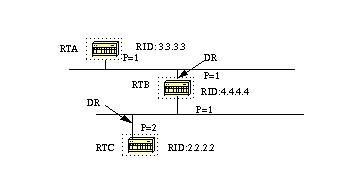
In the above diagram, RTA and RTB have the same interface priority but RTB has a higher RID. RTB would be DR on that segment. RTC has a higher priority than RTB. RTC is DR on that segment.
Building the Adjacency
The adjacency building process takes effect after multiple stages have been fulfilled. Routers that become adjacent will have the exact link-state database. The following is a brief summary of the states an interface passes through before becoming adjacent to another router:-
Down: No information has been received from anybody
on the segment.
-
Attempt: On non-broadcast multi-access clouds such
as Frame Relay and X.25, this state indicates that no recent information has
been received from the neighbor. An effort should be made to contact the
neighbor by sending Hello packets at the reduced rate
PollInterval.
-
Init: The interface has detected a Hello packet
coming from a neighbor but bi-directional communication has not yet been
established.
-
Two-way: There is bi-directional communication with
a neighbor. The router has seen itself in the Hello packets coming from a
neighbor. At the end of this stage the DR and BDR election would have been
done. At the end of the 2way stage, routers will decide whether to proceed in
building an adjacency or not. The decision is based on whether one of the
routers is a DR or BDR or the link is a point-to-point or a virtual
link.
-
Exstart: Routers are trying to establish the initial
sequence number that is going to be used in the information exchange packets.
The sequence number insures that routers always get the most recent
information. One router will become the primary and the other will become
secondary. The primary router will poll the secondary for
information.
-
Exchange: Routers will describe their entire
link-state database by sending database description packets. At this state,
packets could be flooded to other interfaces on the router.
-
Loading: At this state, routers are finalizing the
information exchange. Routers have built a link-state request list and a
link-state retransmission list. Any information that looks incomplete or
outdated will be put on the request list. Any update that is sent will be put
on the retransmission list until it gets acknowledged.
-
Full: At this state, the adjacency is complete. The
neighboring routers are fully adjacent. Adjacent routers will have a similar
link-state database.
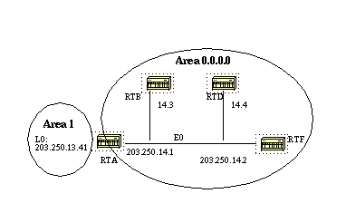
RTA, RTB, RTD, and RTF share a common segment (E0) in area 0.0.0.0. The following are the configs of RTA and RTF. RTB and RTD should have a similar configuration to RTF and will not be included.
The above is a simple example that demonstrates a couple of commands that are very useful in debugging OSPF networks.RTA# hostname RTA interface Loopback0 ip address 203.250.13.41 255.255.255.0 interface Ethernet0 ip address 203.250.14.1 255.255.255.0 router ospf 10 network 203.250.13.41 0.0.0.0 area 1 network 203.250.0.0 0.0.255.255 area 0.0.0.0 RTF# hostname RTF interface Ethernet0 ip address 203.250.14.2 255.255.255.0 router ospf 10 network 203.250.0.0 0.0.255.255 area 0.0.0.0
This command is a quick check to see if all of the interfaces belong to the areas they are supposed to be in. The sequence in which the OSPF network commands are listed is very important. In RTA's configuration, if the "network 203.250.0.0 0.0.255.255 area 0.0.0.0" statement was put before the "network 203.250.13.41 0.0.0.0 area 1" statement, all of the interfaces would be in area 0, which is incorrect because the loopback is in area 1. Let us look at the command's output on RTA, RTF, RTB, and RTD:
RTA#show ip ospf interface e0
Ethernet0 is up, line protocol is up
  Internet Address 203.250.14.1 255.255.255.0, Area 0.0.0.0
  Process ID 10, Router ID 203.250.13.41, Network Type BROADCAST, Cost:
10
  Transmit Delay is 1 sec, State BDR, Priority 1
  Designated Router (ID) 203.250.15.1, Interface address 203.250.14.2
  Backup Designated router (ID) 203.250.13.41, Interface address
203.250.14.1
  Timer intervals configured, Hello 10, Dead 40, Wait 40, Retransmit 5
    Hello due in 0:00:02
  Neighbor Count is 3, Adjacent neighbor count is 3
    Adjacent with neighbor 203.250.15.1  (Designated Router)
Loopback0 is up, line protocol is up
  Internet Address 203.250.13.41 255.255.255.255, Area 1
  Process ID 10, Router ID 203.250.13.41, Network Type LOOPBACK, Cost: 1
  Loopback interface is treated as a stub Host


RTF#show ip ospf interface e0
Ethernet0 is up, line protocol is up
  Internet Address 203.250.14.2 255.255.255.0, Area 0.0.0.0
  Process ID 10, Router ID 203.250.15.1, Network Type BROADCAST, Cost: 10
  Transmit Delay is 1 sec, State DR, Priority 1
  Designated Router (ID) 203.250.15.1, Interface address 203.250.14.2
  Backup Designated router (ID) 203.250.13.41, Interface address
203.250.14.1
  Timer intervals configured, Hello 10, Dead 40, Wait 40, Retransmit 5
    Hello due in 0:00:08
  Neighbor Count is 3, Adjacent neighbor count is 3
    Adjacent with neighbor 203.250.13.41  (Backup Designated Router)


RTD#show ip ospf interface e0
Ethernet0 is up, line protocol is up
  Internet Address 203.250.14.4 255.255.255.0, Area 0.0.0.0
  Process ID 10, Router ID 192.208.10.174, Network Type BROADCAST, Cost:
10
  Transmit Delay is 1 sec, State DROTHER, Priority 1
  Designated Router (ID) 203.250.15.1, Interface address 203.250.14.2
  Backup Designated router (ID) 203.250.13.41, Interface address
203.250.14.1
  Timer intervals configured, Hello 10, Dead 40, Wait 40, Retransmit 5
    Hello due in 0:00:03
  Neighbor Count is 3, Adjacent neighbor count is 2
    Adjacent with neighbor 203.250.15.1  (Designated Router)
    Adjacent with neighbor 203.250.13.41  (Backup Designated Router)


RTB#show ip ospf interface e0
Ethernet0 is up, line protocol is up
  Internet Address 203.250.14.3 255.255.255.0, Area 0.0.0.0
  Process ID 10, Router ID 203.250.12.1, Network Type BROADCAST, Cost: 10
  Transmit Delay is 1 sec, State DROTHER, Priority 1
  Designated Router (ID) 203.250.15.1, Interface address 203.250.14.2
  Backup Designated router (ID) 203.250.13.41, Interface address
203.250.14.1
  Timer intervals configured, Hello 10, Dead 40, Wait 40, Retransmit 5
    Hello due in 0:00:03
  Neighbor Count is 3, Adjacent neighbor count is 2
    Adjacent with neighbor 203.250.15.1  (Designated Router)
    Adjacent with neighbor 203.250.13.41  (Backup Designated Router)
The above output shows very important information. Let us look at RTA's
output. Ethernet0 is in area 0.0.0.0. The process ID is 10 (router ospf 10) and
the router ID is 203.250.13.41. Remember that the RID is the highest IP address
on the box or the loopback interface, calculated at boot time or whenever the
OSPF process is restarted. The state of the interface is BDR. Since all routers
have the same OSPF priority on Ethernet 0 (default is 1), RTF's interface was
elected as DR because of the higher RID. In the same way, RTA was elected as
BDR. RTD and RTB are neither a DR or BDR and their state is DROTHER.Also note the neighbor count and the adjacent count. RTD has three neighbors and is adjacent to two of them, the DR and the BDR. RTF has three neighbors and is adjacent to all of them because it is the DR.
The information about the network type is important and will determine the state of the interface. On broadcast networks such as Ethernet, the election of the DR and BDR should be irrelevant to the end user. It should not matter who the DR or BDR are. In other cases, such as NBMA media such as Frame Relay and X.25, this becomes very important for OSPF to function correctly. Fortunately, with the introduction of point-to-point and point-to-multipoint subinterfaces, DR election is no longer an issue. OSPF over NBMA will be discussed in the next section.
Another command we need to look at is:
Let us look at RTD's output:
The show ip ospf neighbor command shows the state of all the neighbors on a particular segment. Do not be alarmed if the "Neighbor ID" does not belong to the segment you are looking at. In our case 203.250.12.1 and 203.250.15.1 are not on Ethernet0. This is "OK" because the "Neighbor ID" is actually the RID which could be any IP address on the box. RTD and RTB are just neighbors, that is why the state is 2WAY/DROTHER. RTD is adjacent to RTA and RTF and the state is FULL/DR and FULL/BDR.RTD#show ip ospf neighbor Neighbor ID Pri State Dead Time Address Interface 203.250.12.1 1 2WAY/DROTHER 0:00:37 203.250.14.3 Ethernet0 203.250.15.1 1 FULL/DR 0:00:36 203.250.14.2 Ethernet0 203.250.13.41 1 FULL/BDR 0:00:34 203.250.14.1 Ethernet0
Adjacencies on Point-to-Point Interfaces
OSPF will always form an adjacency with the neighbor on the other side of a point-to-point interface such as point-to-point serial lines. There is no concept of DR or BDR. The state of the serial interfaces is point to point.Adjacencies on Non-Broadcast Multi-Access (NBMA) Networks
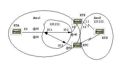
Special care should be taken when configuring OSPF over multi-access non-broadcast medias such as Frame Relay, X.25, ATM. The protocol considers these media like any other broadcast media such as Ethernet. NBMA clouds are usually built in a hub and spoke topology. PVCs or SVCs are laid out in a partial mesh and the physical topology does not provide the multi access that OSPF believes is out there. The selection of the DR becomes an issue because the DR and BDR need to have full physical connectivity with all routers that exist on the cloud. Also, because of the lack of broadcast capabilities, the DR and BDR need to have a static list of all other routers attached to the cloud. This is achieved using the neighbor ip-address [priority number] [poll-interval seconds] command, where the "ip-address" and "priority" are the IP address and the OSPF priority given to the neighbor. A neighbor with priority 0 is considered ineligible for DR election. The "poll-interval" is the amount of time an NBMA interface waits before polling (sending a Hello) to a presumably dead neighbor. The neighbor command applies to routers with a potential of being DRs or BDRs (interface priority not equal to 0). The following diagram shows a network diagram where DR selection is very important: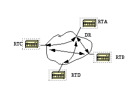
In the above diagram, it is essential for RTA's interface to the cloud to be elected DR. This is because RTA is the only router that has full connectivity to other routers. The election of the DR could be influenced by setting the ospf priority on the interfaces. Routers that do not need to become DRs or BDRs will have a priority of 0 other routers could have a lower priority.
The use of the neighbor command is not covered in depth in this document as this is becoming obsolete with the introduction of new means of setting the interface Network Type to whatever you want irrespective of what the underlying physical media is. This is explained in the next section.
Avoiding DRs and neighbor Command on NBMA
Different methods can be used to avoid the complications of configuring static neighbors and having specific routers becoming DRs or BDRs on the non-broadcast cloud. Specifying which method to use is influenced by whether we are starting the network from scratch or rectifying an already existing design.Point-to-Point Subinterfaces
A subinterface is a logical way of defining an interface. The same physical interface can be split into multiple logical interfaces, with each subinterface being defined as point-to-point. This was originally created in order to better handle issues caused by split horizon over NBMA and vector based routing protocols.A point-to-point subinterface has the properties of any physical point-to-point interface. As far as OSPF is concerned, an adjacency is always formed over a point-to-point subinterface with no DR or BDR election. The following is an illustration of point-to-point subinterfaces:
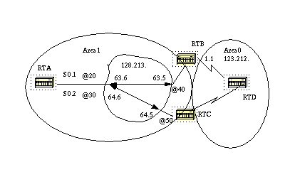
In the above diagram, on RTA, we can split Serial 0 into two point-to-point subinterfaces, S0.1 and S0.2. This way, OSPF will consider the cloud as a set of point-to-point links rather than one multi-access network. The only drawback for the point-to-point is that each segment will belong to a different subnet. This might not be acceptable since some administrators have already assigned one IP subnet for the whole cloud.
Another workaround is to use IP unnumbered interfaces on the cloud. This also might be a problem for some administrators who manage the WAN based on IP addresses of the serial lines. The following is a typical configuration for RTA and RTB:
RTA#

interface Serial 0
 no ip address
 encapsulation frame-relay

interface Serial0.1 point-to-point
 ip address 128.213.63.6 255.255.252.0
 frame-relay interface-dlci 20

interface Serial0.2 point-to-point
 ip address 128.213.64.6 255.255.252.0
 frame-relay interface-dlci 30

router ospf 10
network 128.213.0.0 0.0.255.255 area 1

RTB#

interface Serial 0
 no ip address
 encapsulation frame-relay

interface Serial0.1 point-to-point
 ip address 128.213.63.5 255.255.252.0
 frame-relay interface-dlci 40

interface Serial1
 ip address 123.212.1.1 255.255.255.0

router ospf 10
network 128.213.0.0 0.0.255.255 area 1
network 123.212.0.0 0.0.255.255 area 0
Selecting Interface Network Types
The command used to set the network type of an OSPF interface is:
ip ospf network {broadcast | non-broadcast | point-to-multipoint}
Point-to-Multipoint Interfaces An OSPF point-to-multipoint interface is defined as a numbered point-to-point interface having one or more neighbors. This concept takes the previously discussed point-to-point concept one step further. Administrators do not have to worry about having multiple subnets for each point-to-point link. The cloud is configured as one subnet. This should work well for people who are migrating into the point-to-point concept with no change in IP addressing on the cloud. Also, they would not have to worry about DRs and neighbor statements. OSPF point-to-multipoint works by exchanging additional link-state updates that contain a number of information elements that describe connectivity to the neighboring routers.
Note that no static frame relay map statements were configured; this is because Inverse ARP takes care of the DLCI to IP address mapping. Let us look at some of show ip ospf interface and show ip ospf route outputs:RTA# interface Loopback0 ip address 200.200.10.1 255.255.255.0 interface Serial0 ip address 128.213.10.1 255.255.255.0 encapsulation frame-relay ip ospf network point-to-multipoint router ospf 10 network 128.213.0.0 0.0.255.255 area 1 RTB# interface Serial0 ip address 128.213.10.2 255.255.255.0 encapsulation frame-relay ip ospf network point-to-multipoint interface Serial1 ip address 123.212.1.1 255.255.255.0 router ospf 10 network 128.213.0.0 0.0.255.255 area 1 network 123.212.0.0 0.0.255.255 area 0
RTA#show ip ospf interface s0
Serial0 is up, line protocol is up
  Internet Address 128.213.10.1 255.255.255.0, Area 0
  Process ID 10, Router ID 200.200.10.1, Network Type
POINT_TO_MULTIPOINT, Cost: 64
  Transmit Delay is 1 sec, State POINT_TO_MULTIPOINT,
  Timer intervals configured, Hello 30, Dead 120, Wait 120, Retransmit 5
    Hello due in 0:00:04
  Neighbor Count is 2, Adjacent neighbor count is 2
    Adjacent with neighbor 195.211.10.174
    Adjacent with neighbor 128.213.63.130

RTA#show ip ospf neighbor

Neighbor ID     Pri   State           Dead Time   Address         Interface
128.213.10.3      1   FULL/  -        0:01:35     128.213.10.3    Serial0
128.213.10.2      1   FULL/  -        0:01:44     128.213.10.2    Serial0

RTB#show ip ospf interface s0

Serial0 is up, line protocol is up
  Internet Address 128.213.10.2 255.255.255.0, Area 0
  Process ID 10, Router ID 128.213.10.2, Network Type
POINT_TO_MULTIPOINT, Cost: 64
  Transmit Delay is 1 sec, State POINT_TO_MULTIPOINT,
  Timer intervals configured, Hello 30, Dead 120, Wait 120, Retransmit 5
    Hello due in 0:00:14
  Neighbor Count is 1, Adjacent neighbor count is 1
    Adjacent with neighbor 200.200.10.1

RTB#show ip ospf neighbor

Neighbor ID     Pri   State           Dead Time   Address         Interface
200.200.10.1      1   FULL/  -        0:01:52     128.213.10.1    Serial0
The only drawback for point-to-multipoint is that it generates multiple
Hosts routes (routes with mask 255.255.255.255) for all the neighbors. Note the
Host routes in the following IP routing table for RTB:
RTB#show ip route
 Codes: C - connected, S - static, I - IGRP, R - RIP, M - mobile, B - BGP
        D - EIGRP, EX - EIGRP external, O - OSPF, IA - OSPF inter area
        E1 - OSPF external type 1, E2 - OSPF external type 2, E - EGP
        i - IS-IS, L1 - IS-IS level-1, L2 - IS-IS level-2, * - candidate default

 Gateway of last resort is not set

      200.200.10.0 255.255.255.255 is subnetted, 1 subnets
 O       200.200.10.1 [110/65] via 128.213.10.1,  Serial0
         128.213.0.0 is variably subnetted, 3 subnets, 2 masks
 O    128.213.10.3 255.255.255.255
            [110/128] via 128.213.10.1, 00:00:00, Serial0
 O    128.213.10.1 255.255.255.255
            [110/64] via 128.213.10.1, 00:00:00, Serial0
 C       128.213.10.0 255.255.255.0 is directly connected, Serial0
      123.0.0.0 255.255.255.0 is subnetted, 1 subnets
 C       123.212.1.0 is directly connected, Serial1

 RTC#show ip route

      200.200.10.0 255.255.255.255 is subnetted, 1 subnets
 O       200.200.10.1 [110/65] via 128.213.10.1, Serial1
      128.213.0.0 is variably subnetted, 4 subnets, 2 masks
 O       128.213.10.2 255.255.255.255 [110/128] via 128.213.10.1,Serial1
 O       128.213.10.1 255.255.255.255 [110/64] via 128.213.10.1, Serial1
 C       128.213.10.0 255.255.255.0 is directly connected, Serial1
      123.0.0.0 255.255.255.0 is subnetted, 1 subnets
 O       123.212.1.0 [110/192] via 128.213.10.1, 00:14:29, Serial1
Note that in RTC's IP routing table, network 123.212.1.0 is reachable
via next hop 128.213.10.1 and not via 128.213.10.2 as you normally see over
Frame Relay clouds sharing the same subnet. This is one advantage of the
point-to-multipoint configuration because you do not need to resort to static
mapping on RTC to be able to reach next hop 128.213.10.2. Broadcast Interfaces
This approach is a workaround for using the "neighbor" command which statically lists all existing neighbors. The interface will be logically set to broadcast and will behave as if the router were connected to a LAN. DR and BDR election will still be performed so special care should be taken to assure either a full mesh topology or a static selection of the DR based on the interface priority. The command that sets the interface to broadcast is:
ip ospf network broadcast
OSPF and Route Summarization
Summarizing is the consolidation of multiple routes into one single advertisement. This is normally done at the boundaries of Area Border Routers (ABRs). Although summarization could be configured between any two areas, it is better to summarize in the direction of the backbone. This way the backbone receives all the aggregate addresses and in turn will injects them, already summarized, into other areas. There are two types of summarization:-
Inter-area route summarization
-
External route summarization
Inter-Area Route Summarization
Inter-area route summarization is done on ABRs and it applies to routes from within the AS. It does not apply to external routes injected into OSPF via redistribution. In order to take advantage of summarization, network numbers in areas should be assigned in a contiguous way to be able to lump these addresses into one range. To specify an address range, perform the following task in router configuration mode:Where the "area-id" is the area containing networks to be summarized. The "address" and "mask" will specify the range of addresses to be summarized in one range. The following is an example of summarization:area area-id range address mask
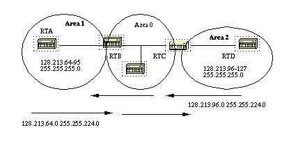
In the above diagram, RTB is summarizing the range of subnets from 128.213.64.0 to 128.213.95.0 into one range: 128.213.64.0 255.255.224.0. This is achieved by masking the first three left most bits of 64 using a mask of 255.255.224.0. In the same way, RTC is generating the summary address 128.213.96.0 255.255.224.0 into the backbone. Note that this summarization was successful because we have two distinct ranges of subnets, 64-95 and 96-127.
It would be hard to summarize if the subnets between area 1 and area 2 were overlapping. The backbone area would receive summary ranges that overlap and routers in the middle would not know where to send the traffic based on the summary address.
The following is the relative configuration of RTB:
Prior to Cisco IOS® Software Release 12.1(6), it was recommended to manually configure, on the ABR, a discard static route for the summary address in order to prevent possible routing loops. For the summary route shown above, you can use this command:RTB# router ospf 100 area 1 range 128.213.64.0 255.255.224.0
In IOS 12.1(6) and higher, the discard route is automatically generated by default. If for any reason you don't want to use this discard route, you can configure the following commands under router ospf:ip route 128.213.64.0 255.255.224.0 null0
or[no] discard-route internal
[no] discard-route external
Note about summary address metric calculation: RFC 1583 called for calculating the metric for summary routes based on the minimum
metric of the component paths available. RFC 2178 (now obsoleted by RFC 2328) changed the specified method for calculating metrics for summary routes so the component of the summary with the maximum (or largest) cost would determine the cost of the summary.
Prior to IOS 12.0, Cisco was compliant with the then-current RFC 1583. As of IOS 12.0, Cisco changed the behavior of OSPF to be compliant with the new standard, RFC 2328. This situation created the possibility of sub-optimal routing if all of the ABRs in an area were not upgraded to the new code at the same time. In order to address this potential problem, a command has been added to the OSPF configuration of Cisco IOS that allows you to selectively disable compatibility with RFC 2328. The new configuration command is under router ospf, and has the following syntax:
The default setting is compatible with RFC 1583. This command is available in the following versions of IOS:[no] compatible rfc1583
-
12.1(03)DC
-
12.1(03)DB
-
12.001(001.003) - 12.1 Mainline
-
12.1(01.03)T - 12.1 T-Train
-
12.000(010.004) - 12.0 Mainline
-
12.1(01.03)E - 12.1 E-Train
-
12.1(01.03)EC
-
12.0(10.05)W05(18.00.10)
-
12.0(10.05)SC
External Route Summarization
External route summarization is specific to external routes that are injected into OSPF via redistribution. Also, make sure that external ranges that are being summarized are contiguous. Summarization overlapping ranges from two different routers could cause packets to be sent to the wrong destination. Summarization is done via the following router ospf subcommand:This command is effective only on ASBRs doing redistribution into OSPF.summary-address ip-address mask
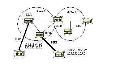
In the above diagram, RTA and RTD are injecting external routes into OSPF by redistribution. RTA is injecting subnets in the range 128.213.64-95 and RTD is injecting subnets in the range 128.213.96-127. In order to summarize the subnets into one range on each router we can do the following:
This will cause RTA to generate one external route 128.213.64.0 255.255.224.0 and will cause RTD to generate 128.213.96.0 255.255.224.0.RTA# router ospf 100 summary-address 128.213.64.0 255.255.224.0 redistribute bgp 50 metric 1000 subnets RTD# router ospf 100 summary-address 128.213.96.0 255.255.224.0 redistribute bgp 20 metric 1000 subnets
Note that the summary-address command has no effect if used on RTB because RTB is not doing the redistribution into OSPF.
Stub Areas
OSPF allows certain areas to be configured as stub areas. External networks, such as those redistributed from other protocols into OSPF, are not allowed to be flooded into a stub area. Routing from these areas to the outside world is based on a default route. Configuring a stub area reduces the topological database size inside an area and reduces the memory requirements of routers inside that area.An area could be qualified a stub when there is a single exit point from that area or if routing to outside of the area does not have to take an optimal path. The latter description is just an indication that a stub area that has multiple exit points, will have one or more area border routers injecting a default into that area. Routing to the outside world could take a sub-optimal path in reaching the destination by going out of the area via an exit point which is farther to the destination than other exit points.
Other stub area restrictions are that a stub area cannot be used as a transit area for virtual links. Also, an ASBR cannot be internal to a stub area. These restrictions are made because a stub area is mainly configured not to carry external routes and any of the above situations cause external links to be injected in that area. The backbone, of course, cannot be configured as stub.
All OSPF routers inside a stub area have to be configured as stub routers. This is because whenever an area is configured as stub, all interfaces that belong to that area will start exchanging Hello packets with a flag that indicates that the interface is stub. Actually this is just a bit in the Hello packet (E bit) that gets set to 0. All routers that have a common segment have to agree on that flag. If they don't, then they will not become neighbors and routing will not take effect.
An extension to stub areas is what is called "totally stubby areas". Cisco indicates this by adding a "no-summary" keyword to the stub area configuration. A totally stubby area is one that blocks external routes and summary routes (inter-area routes) from going into the area. This way, intra-area routes and the default of 0.0.0.0 are the only routes injected into that area.
The command that configures an area as stub is:
and the command that configures a default-cost into an area is:areastub [no-summary]
If the cost is not set using the above command, a cost of 1 will be advertised by the ABR.area area-id default-cost cost
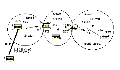
Assume that area 2 is to be configured as a stub area. The following example will show the routing table of RTE before and after configuring area 2 as stub.
RTC#

 interface Ethernet 0
  ip address 203.250.14.1 255.255.255.0

 interface Serial1
  ip address 203.250.15.1 255.255.255.252

 router ospf 10
  network 203.250.15.0 0.0.0.255 area 2
  network 203.250.14.0 0.0.0.255 area 0
 RTE#show ip route
 Codes: C - connected, S - static, I - IGRP, R - RIP, M - mobile, B - BGP
        D - EIGRP, EX - EIGRP external, O - OSPF, IA - OSPF inter area
        E1 - OSPF external type 1, E2 - OSPF external type 2, E - EGP
        i - IS-IS, L1 - IS-IS level-1, L2 - IS-IS level-2, * - candidate default

 Gateway of last resort is not set

      203.250.15.0 255.255.255.252 is subnetted, 1 subnets
 C       203.250.15.0 is directly connected, Serial0
 O IA 203.250.14.0 [110/74] via 203.250.15.1, 00:06:31, Serial0
      128.213.0.0 is variably subnetted, 2 subnets, 2 masks
 O E2    128.213.64.0 255.255.192.0
            [110/10] via 203.250.15.1, 00:00:29, Serial0
 O IA    128.213.63.0 255.255.255.252
            [110/84] via 203.250.15.1, 00:03:57, Serial0
      131.108.0.0 255.255.255.240 is subnetted, 1 subnets
 O       131.108.79.208 [110/74] via 203.250.15.1, 00:00:10, Serial0
RTE has learned the inter-area routes (O IA) 203.250.14.0 and
128.213.63.0 and it has learned the intra-area route (O) 131.108.79.208 and the
external route (O E2) 128.213.64.0.If we configure area 2 as stub, we need to do the following:
Note that the stub command is configured on RTE also, otherwise RTE will never become a neighbor to RTC. The default cost was not set, so RTC will advertise 0.0.0.0 to RTE with a metric of 1.RTC# interface Ethernet 0 ip address 203.250.14.1 255.255.255.0 interface Serial1 ip address 203.250.15.1 255.255.255.252 router ospf 10 network 203.250.15.0 0.0.0.255 area 2 network 203.250.14.0 0.0.0.255 area 0 area 2 stub RTE# interface Serial1 ip address 203.250.15.2 255.255.255.252 router ospf 10 network 203.250.15.0 0.0.0.255 area 2 area 2 stub
RTE#show ip route
 Codes: C - connected, S - static, I - IGRP, R - RIP, M - mobile, B - BGP
        D - EIGRP, EX - EIGRP external, O - OSPF, IA - OSPF inter area
        E1 - OSPF external type 1, E2 - OSPF external type 2, E - EGP
        i - IS-IS, L1 - IS-IS level-1, L2 - IS-IS level-2, * - candidate default

 Gateway of last resort is 203.250.15.1 to network 0.0.0.0

      203.250.15.0 255.255.255.252 is subnetted, 1 subnets
 C       203.250.15.0 is directly connected, Serial0
 O IA 203.250.14.0 [110/74] via 203.250.15.1, 00:26:58, Serial0
      128.213.0.0 255.255.255.252 is subnetted, 1 subnets
 O IA    128.213.63.0 [110/84] via 203.250.15.1, 00:26:59, Serial0
      131.108.0.0 255.255.255.240 is subnetted, 1 subnets
 O       131.108.79.208 [110/74] via 203.250.15.1, 00:26:59, Serial0
 O*IA 0.0.0.0 0.0.0.0 [110/65] via 203.250.15.1, 00:26:59, Serial0
Note that all the routes show up except the external routes which were
replaced by a default route of 0.0.0.0. The cost of the route happened to be 65
(64 for a T1 line + 1 advertised by RTC). We will now configure area 2 to be totally stubby, and change the default cost of 0.0.0.0 to 10.
RTC#

 interface Ethernet 0
  ip address 203.250.14.1 255.255.255.0

 interface Serial1
  ip address 203.250.15.1 255.255.255.252

 router ospf 10
  network 203.250.15.0 0.0.0.255 area 2
  network 203.250.14.0 0.0.0.255 area 0
  area 2 stub no-summary
  area 2 default cost 10


 RTE#show ip route

 Codes: C - connected, S - static, I - IGRP, R - RIP, M - mobile, B - BGP
        D - EIGRP, EX - EIGRP external, O - OSPF, IA - OSPF inter area
        E1 - OSPF external type 1, E2 - OSPF external type 2, E - EGP
        i - IS-IS, L1 - IS-IS level-1, L2 - IS-IS level-2, * - candidate default

 Gateway of last resort is not set

      203.250.15.0 255.255.255.252 is subnetted, 1 subnets
 C       203.250.15.0 is directly connected, Serial0
      131.108.0.0 255.255.255.240 is subnetted, 1 subnets
 O       131.108.79.208 [110/74] via 203.250.15.1, 00:31:27, Serial0
 O*IA 0.0.0.0 0.0.0.0 [110/74] via 203.250.15.1, 00:00:00, Serial0
Note that the only routes that show up are the intra-area routes (O)
and the default-route 0.0.0.0. The external and inter-area routes have been
blocked. The cost of the default route is now 74 (64 for a T1 line + 10
advertised by RTC). No configuration is needed on RTE in this case. The area is
already stub, and the no-summary command does not
affect the Hello packet at all as the stub command does. Redistributing Routes into OSPF
Redistributing routes into OSPF from other routing protocols or from static will cause these routes to become OSPF external routes. To redistribute routes into OSPF, use the following command in router configuration mode:redistribute protocol [process-id] [metric value] [metric-type value] [route-map map-tag] [subnets]
Note: The above command should be on one line.
The protocol and process-id are the protocol that we are injecting into
OSPF and its process-id if it exits. The metric is the cost we are assigning to
the external route. If no metric is specified, OSPF puts a default value of 20
when redistributing routes from all protocols except BGP routes, which get a
metric of 1. The metric-type is discussed in the next paragraph. The route-map is a method used to control the redistribution of routes between routing domains. The format of a route map is:
When redistributing routes into OSPF, only routes that are not subnetted are redistributed if the subnets keyword is not specified.route-map map-tag [[permit | deny] | [sequence-number]]
E1 vs. E2 External Routes
External routes fall under two categories, external type 1 and external type 2. The difference between the two is in the way the cost (metric) of the route is being calculated. The cost of a type 2 route is always the external cost, irrespective of the interior cost to reach that route. A type 1 cost is the addition of the external cost and the internal cost used to reach that route. A type 1 route is always preferred over a type 2 route for the same destination. This is illustrated in the following diagram: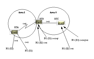
As the above diagram shows, RTA is redistributing two external routes into OSPF. N1 and N2 both have an external cost of x. The only difference is that N1 is redistributed into OSPF with a metric-type 1 and N2 is redistributed with a metric-type 2. If we follow the routes as they flow from Area 1 to Area 0, the cost to reach N2 as seen from RTB or RTC will always be x. The internal cost along the way is not considered. On the other hand, the cost to reach N1 is incremented by the internal cost. The cost is x+y as seen from RTB and x+y+z as seen from RTC.
If the external routes are both type 2 routes and the external costs to the destination network are equal, then the path with the lowest cost to the ASBR is selected as the best path.
Unless otherwise specified, the default external type given to external routes is type 2.

Suppose we added two static routes pointing to E0 on RTC: 16.16.16.0 255.255.255.0 (the /24 notation indicates a 24 bit mask starting from the far left) and 128.213.0.0 255.255.0.0. The following shows the different behaviors when different parameters are used in the redistribute command on RTC:
The following is the output of show ip route on RTE:RTC# interface Ethernet0 ip address 203.250.14.2 255.255.255.0 interface Serial1 ip address 203.250.15.1 255.255.255.252 router ospf 10 redistribute static network 203.250.15.0 0.0.0.255 area 2 network 203.250.14.0 0.0.0.255 area 0 ip route 16.16.16.0 255.255.255.0 Ethernet0 ip route 128.213.0.0 255.255.0.0 Ethernet0 RTE# interface Serial0 ip address 203.250.15.2 255.255.255.252 router ospf 10 network 203.250.15.0 0.0.0.255 area 2
RTE#show ip route
 Codes: C - connected, S - static, I - IGRP, R - RIP, M - mobile, B - BGP
        D - EIGRP, EX - EIGRP external, O - OSPF, IA - OSPF inter area
        E1 - OSPF external type 1, E2 - OSPF external type 2, E - EGP
        i - IS-IS, L1 - IS-IS level-1, L2 - IS-IS level-2, * - candidate default

 Gateway of last resort is not set

      203.250.15.0 255.255.255.252 is subnetted, 1 subnets
 C       203.250.15.0 is directly connected, Serial0
 O IA 203.250.14.0 [110/74] via 203.250.15.1, 00:02:31, Serial0
 O E2 128.213.0.0 [110/20] via 203.250.15.1, 00:02:32, Serial0
Note that the only external route that has appeared is 128.213.0.0,
because we did not use the subnet keyword. Remember
that if the subnet keyword is not used, only routes
that are not subnetted will be redistributed. In our case 16.16.16.0 is a class
A route that is subnetted and it did not get redistributed. Since the metric keyword was not used (or a default-metric statement under router OSPF), the
cost allocated to the external route is 20 (the default is 1 for BGP). If we
use the following:
redistribute static metric 50 subnets

RTE#show ip route
Codes: C - connected, S - static, I - IGRP, R - RIP, M
- mobile, B - BGP
        D - EIGRP, EX - EIGRP external, O - OSPF, IA - OSPF inter area
        E1 - OSPF external type 1, E2 - OSPF external type 2, E - EGP
        i - IS-IS, L1 - IS-IS level-1, L2 - IS-IS level-2, * - candidate default

 Gateway of last resort is not set

      16.0.0.0 255.255.255.0 is subnetted, 1 subnets
 O E2    16.16.16.0 [110/50] via 203.250.15.1, 00:00:02, Serial0
      203.250.15.0 255.255.255.252 is subnetted, 1 subnets
 C       203.250.15.0 is directly connected, Serial0
 O IA 203.250.14.0 [110/74] via 203.250.15.1, 00:00:02, Serial0
 O E2 128.213.0.0 [110/50] via 203.250.15.1, 00:00:02, Serial0
Note that 16.16.16.0 has shown up now and the cost to external routes
is 50. Since the external routes are of type 2 (E2), the internal cost has not
been added. Suppose now, we change the type to E1:
redistribute static metric 50 metric-type 1 subnets

RTE#show ip route
 Codes: C - connected, S - static, I - IGRP, R - RIP, M - mobile, B - BGP
        D - EIGRP, EX - EIGRP external, O - OSPF, IA - OSPF inter area
        E1 - OSPF external type 1, E2 - OSPF external type 2, E - EGP
        i - IS-IS, L1 - IS-IS level-1, L2 - IS-IS level-2, * - candidate default

 Gateway of last resort is not set

      16.0.0.0 255.255.255.0 is subnetted, 1 subnets
 O E1    16.16.16.0 [110/114] via 203.250.15.1, 00:04:20, Serial0
      203.250.15.0 255.255.255.252 is subnetted, 1 subnets
 C       203.250.15.0 is directly connected, Serial0
 O IA 203.250.14.0 [110/74] via 203.250.15.1, 00:09:41, Serial0
 O E1 128.213.0.0 [110/114] via 203.250.15.1, 00:04:21, Serial0
Note that the type has changed to E1 and the cost has been incremented
by the internal cost of S0 which is 64, the total cost is 64+50=114.Assume that we add a route map to RTC's configuration, we will get the following:
The route map above will only permit 128.213.0.0 to be redistributed into OSPF and will deny the rest. This is why 16.16.16.0 does not show up in RTE's routing table anymore.RTC# interface Ethernet0 ip address 203.250.14.2 255.255.255.0 interface Serial1 ip address 203.250.15.1 255.255.255.252 router ospf 10 redistribute static metric 50 metric-type 1 subnets route-map STOPUPDATE network 203.250.15.0 0.0.0.255 area 2 network 203.250.14.0 0.0.0.255 area 0 ip route 16.16.16.0 255.255.255.0 Ethernet0 ip route 128.213.0.0 255.255.0.0 Ethernet0 access-list 1 permit 128.213.0.0 0.0.255.255 route-map STOPUPDATE permit 10 match ip address 1
RTE#show ip route
 Codes: C - connected, S - static, I - IGRP, R - RIP, M - mobile, B - BGP
        D - EIGRP, EX - EIGRP external, O - OSPF, IA - OSPF inter area
        E1 - OSPF external type 1, E2 - OSPF external type 2, E - EGP
        i - IS-IS, L1 - IS-IS level-1, L2 - IS-IS level-2, * - candidate default

 Gateway of last resort is not set

      203.250.15.0 255.255.255.252 is subnetted, 1 subnets
 C       203.250.15.0 is directly connected, Serial0
 O IA 203.250.14.0 [110/74] via 203.250.15.1, 00:00:04, Serial0
 O E1 128.213.0.0 [110/114] via 203.250.15.1, 00:00:05, Serial0
Redistributing OSPF into Other Protocols
Use of a Valid Metric
Whenever you redistribute OSPF into other protocols, you have to respect the rules of those protocols. In particular, the metric applied should match the metric used by that protocol. For example, the RIP metric is a hop count ranging between 1 and 16, where 1 indicates that a network is one hop away and 16 indicates that the network is unreachable. On the other hand IGRP and EIGRP require a metric of the form:default-metric bandwidth delay reliability loading mtu
VLSM
Another issue to consider is VLSM (Variable Length Subnet Guide)(Appendix C). OSPF can carry multiple subnet information for the same major net, but other protocols such as RIP and IGRP (EIGRP is OK with VLSM) cannot. If the same major net crosses the boundaries of an OSPF and RIP domain, VLSM information redistributed into RIP or IGRP will be lost and static routes will have to be configured in the RIP or IGRP domains. The following example illustrates this problem: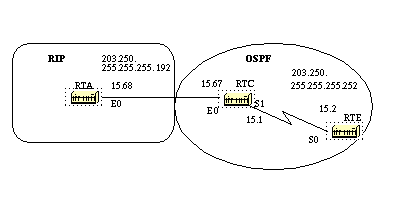
In the above diagram, RTE is running OSPF and RTA is running RIP. RTC is doing the redistribution between the two protocols. The problem is that the class C network 203.250.15.0 is variably subnetted, it has two different masks 255.255.255.252 and 255.255.255.192. Let us look at the configuration and the routing tables of RTE and RTA:
RTA#
 interface Ethernet0
  ip address 203.250.15.68 255.255.255.192
 router rip
  network 203.250.15.0
 RTC#
 interface Ethernet0
  ip address 203.250.15.67 255.255.255.192

 interface Serial1
  ip address 203.250.15.1 255.255.255.252
 router ospf 10
 redistribute rip metric 10 subnets
  network 203.250.15.0 0.0.0.255 area 0
 router rip
  redistribute ospf 10 metric 2
  network 203.250.15.0

 RTE#show ip route
 Codes: C - connected, S - static, I - IGRP, R - RIP, M - mobile, B - BGP
        D - EIGRP, EX - EIGRP external, O - OSPF, IA - OSPF inter area
        E1 - OSPF external type 1, E2 - OSPF external type 2, E - EGP
        i - IS-IS, L1 - IS-IS level-1, L2 - IS-IS level-2, * - candidate default

 Gateway of last resort is not set

      203.250.15.0 is variably subnetted, 2 subnets, 2 masks
 C       203.250.15.0 255.255.255.252 is directly connected, Serial0
 O       203.250.15.64 255.255.255.192
            [110/74] via 203.250.15.1, 00:15:55, Serial0
 RTA#show ip route
 Codes: C - connected, S - static, I - IGRP, R - RIP, M - mobile, B - BGP
        D - EIGRP, EX - EIGRP external, O - OSPF, IA - OSPF inter area
        E1 - OSPF external type 1, E2 - OSPF external type 2, E - EGP
        i - IS-IS, L1 - IS-IS level-1, L2 - IS-IS level-2, * - candidate default

 Gateway of last resort is not set

      203.250.15.0 255.255.255.192 is subnetted, 1 subnets
 C       203.250.15.64 is directly connected, Ethernet0
Note that RTE has recognized that 203.250.15.0 has two subnets while
RTA thinks that it has only one subnet (the one configured on the interface).
Information about subnet 203.250.15.0 255.255.255.252 is lost in the RIP
domain. In order to reach that subnet, a static route needs to be configured on
RTA: This way RTA will be able to reach the other subnets.RTA# interface Ethernet0 ip address 203.250.15.68 255.255.255.192 router rip network 203.250.15.0 ip route 203.250.15.0 255.255.255.0 203.250.15.67
Mutual Redistribution
Mutual redistribution between protocols should be done very carefully and in a controlled manner. Incorrect configuration could lead to potential looping of routing information. A rule of thumb for mutual redistribution is not to allow information learned from a protocol to be injected back into the same protocol. Passive interfaces and distribute lists should be applied on the redistributing routers. Filtering information with link-state protocols such as OSPF is a tricky business. Distribute-list out works on the ASBR to filter redistributed routes into other protocols. Distribute-list in works on any router to prevent routes from being put in the routing table, but it does not prevent link-state packets from being propagated, downstream routers would still have the routes. It is better to avoid OSPF filtering as much as possible if filters can be applied on the other protocols to prevent loops.
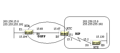
To illustrate, suppose RTA, RTC, and RTE are running RIP. RTC and RTA are also running OSPF. Both RTC and RTA are doing redistribution between RIP and OSPF. Let us assume that you do not want the RIP coming from RTE to be injected into the OSPF domain so you put a passive interface for RIP on E0 of RTC. However, you have allowed the RIP coming from RTA to be injected into OSPF. Here is the outcome:
Note: Do not use the following configuration.
RTE#
 interface Ethernet0
  ip address 203.250.15.130 255.255.255.192

 interface Serial0
  ip address 203.250.15.2 255.255.255.192

 router rip
  network 203.250.15.0


RTC#
 interface Ethernet0
  ip address 203.250.15.67 255.255.255.192

 interface Serial1
  ip address 203.250.15.1 255.255.255.192

 router ospf 10
  redistribute rip metric 10 subnets
  network 203.250.15.0 0.0.0.255 area 0

 router rip
  redistribute ospf 10 metric 2
  passive-interface Ethernet0
  network 203.250.15.0


RTA#
interface Ethernet0
 ip address 203.250.15.68 255.255.255.192

router ospf 10
 redistribute rip metric 10 subnets
 network 203.250.15.0 0.0.0.255 area 0


router rip
 redistribute ospf 10 metric 1
 network 203.250.15.0


RTC#show ip route
 Codes: C - connected, S - static, I - IGRP, R - RIP, M - mobile, B - BGP
        D - EIGRP, EX - EIGRP external, O - OSPF, IA - OSPF inter area
        E1 - OSPF external type 1, E2 - OSPF external type 2, E - EGP
        i - IS-IS, L1 - IS-IS level-1, L2 - IS-IS level-2, * - candidate default

 Gateway of last resort is not set

      203.250.15.0 255.255.255.192 is subnetted, 4 subnets
 C       203.250.15.0 is directly connected, Serial1
 C       203.250.15.64 is directly connected, Ethernet0
 R       203.250.15.128 [120/1] via 203.250.15.68, 00:01:08, Ethernet0
                        [120/1] via 203.250.15.2, 00:00:11, Serial1
 O       203.250.15.192 [110/20] via 203.250.15.68, 00:21:41, Ethernet0
Note that RTC has two paths to reach 203.250.15.128 subnet: Serial 1
and Ethernet 0 (E0 is obviously the wrong path). This happened because RTC gave
that entry to RTA via OSPF and RTA gave it back via RIP because RTA did not
learn it via RIP. This example is a very small scale of loops that can occur
because of an incorrect configuration. In large networks this situation gets
even more aggravated.In order to fix the situation in our example, you could stop RIP from being sent on RTA's Ethernet 0 via a passive interface. This might not be suitable in case some routers on the Ethernet are RIP only routers. In this case, you could allow RTC to send RIP on the Ethernet; this way RTA will not send it back on the wire because of split horizon (this might not work on NBMA media if split horizon is off). Split horizon does not allow updates to be sent back on the same interface they were learned from (via the same protocol). Another good method is to apply distribute-lists on RTA to deny subnets learned via OSPF from being put back into RIP on the Ethernet. The latter is the one we will be using:
And the output of RTC's routing table would be:RTA# interface Ethernet0 ip address 203.250.15.68 255.255.255.192 router ospf 10 redistribute rip metric 10 subnets network 203.250.15.0 0.0.0.255 area 0 router rip redistribute ospf 10 metric 1 network 203.250.15.0 distribute-list 1 out ospf 10
RTF#show ip route
 Codes: C - connected, S - static, I - IGRP, R - RIP, M - mobile, B - BGP
        D - EIGRP, EX - EIGRP external, O - OSPF, IA - OSPF inter area
        E1 - OSPF external type 1, E2 - OSPF external type 2, E - EGP
        i - IS-IS, L1 - IS-IS level-1, L2 - IS-IS level-2, * - candidate default

 Gateway of last resort is not set

      203.250.15.0 255.255.255.192 is subnetted, 4 subnets
 C       203.250.15.0 is directly connected, Serial1
 C       203.250.15.64 is directly connected, Ethernet0
 R       203.250.15.128 [120/1] via 203.250.15.2, 00:00:19, Serial1
 O       203.250.15.192 [110/20] via 203.250.15.68, 00:21:41, Ethernet0
Injecting Defaults into OSPF
An autonomous system boundary router (ASBR) can be forced to generate a default route into the OSPF domain. As discussed earlier, a router becomes an ASBR whenever routes are redistributed into an OSPF domain. However, an ASBR does not, by default, generate a default route into the OSPF routing domain.To have OSPF generate a default route use the following:
default-information originate [always] [metric metric-value]
[metric-type type-value] [route-map map-name]
Note: The above command should be on one line.
There are two ways to generate a default. The first is to advertise
0.0.0.0 inside the domain, but only if the ASBR itself already has a default
route. The second is to advertise 0.0.0.0 regardless whether the ASBR has a
default route. The latter can be set by adding the keyword always. You should be careful when using the always keyword. If your router advertises a default (0.0.0.0)
inside the domain and does not have a default itself or a path to reach the
destinations, routing will be broken. The metric and metric type are the cost and type (E1 or E2) assigned to the default route. The route map specifies the set of conditions that need to be satisfied in order for the default to be generated.
Assume that RTE is injecting a default-route 0.0.0.0 into RIP. RTC will have a gateway of last resort of 203.250.15.2. RTC will not propagate the default to RTA until we configure RTC with a default-information originate command.
RTC#show ip route
 Codes: C - connected, S - static, I - IGRP, R - RIP, M - mobile, B - BGP
        D - EIGRP, EX - EIGRP external, O - OSPF, IA - OSPF inter area
        E1 - OSPF external type 1, E2 - OSPF external type 2, E - EGP
        i - IS-IS, L1 - IS-IS level-1, L2 - IS-IS level-2, * - candidate default

 Gateway of last resort is 203.250.15.2 to network 0.0.0.0

      203.250.15.0 255.255.255.192 is subnetted, 4 subnets
 C       203.250.15.0 is directly connected, Serial1
 C       203.250.15.64 is directly connected, Ethernet0
 R       203.250.15.128 [120/1] via 203.250.15.2, 00:00:17, Serial1
 O       203.250.15.192 [110/20] via 203.250.15.68, 2d23, Ethernet0
 R*   0.0.0.0 0.0.0.0 [120/1] via 203.250.15.2, 00:00:17, Serial1
             [120/1] via 203.250.15.68, 00:00:32, Ethernet0
 RTC#

 interface Ethernet0
  ip address 203.250.15.67 255.255.255.192

 interface Serial1
  ip address 203.250.15.1 255.255.255.192

 router ospf 10
  redistribute rip metric 10 subnets
  network 203.250.15.0 0.0.0.255 area 0
  default-information originate metric 10


 router rip
  redistribute ospf 10 metric 2
  passive-interface Ethernet0
  network 203.250.15.0

RTA#show ip route

 Codes: C - connected, S - static, I - IGRP, R - RIP, M - mobile, B - BGP
        D - EIGRP, EX - EIGRP external, O - OSPF, IA - OSPF inter area
        E1 - OSPF external type 1, E2 - OSPF external type 2, E - EGP
        i - IS-IS, L1 - IS-IS level-1, L2 - IS-IS level-2, * - candidate default

 Gateway of last resort is 203.250.15.67 to network 0.0.0.0

      203.250.15.0 255.255.255.192 is subnetted, 4 subnets
 O       203.250.15.0 [110/74] via 203.250.15.67, 2d23, Ethernet0
 C       203.250.15.64 is directly connected, Ethernet0
 O E2    203.250.15.128 [110/10] via 203.250.15.67, 2d23, Ethernet0
 C       203.250.15.192 is directly connected, Ethernet1
 O*E2 0.0.0.0 0.0.0.0 [110/10] via 203.250.15.67, 00:00:17, Ethernet0
Note that RTA has learned 0.0.0.0 as an external route with metric 10.
The gateway of last resort is set to 203.250.15.67 as expected. OSPF Design Tips
The OSPF RFC (1583) did not specify any guidelines for the number of routers in an area or number the of neighbors per segment or what is the best way to architect a network. Different people have different approaches to designing OSPF networks. The important thing to remember is that any protocol can fail under pressure. The idea is not to challenge the protocol but rather to work with it in order to get the best behavior. The following are a list of things to consider.Number of Routers per Area
The maximum number of routers per area depends on several factors, including the following:-
What kind of area do you have?
-
What kind of CPU power do you have in that area?
-
What kind of media?
-
Will you be running OSPF in NBMA mode?
-
Is your NBMA network meshed?
-
Do you have a lot of external LSAs in the network?
-
Are other areas well summarized?
Number of Neighbors
The number of routers connected to the same LAN is also important. Each LAN has a DR and BDR that build adjacencies with all other routers. The fewer neighbors that exist on the LAN, the smaller the number of adjacencies a DR or BDR have to build. That depends on how much power your router has. You could always change the OSPF priority to select your DR. Also if possible, try to avoid having the same router be the DR on more than one segment. If DR selection is based on the highest RID, then one router could accidently become a DR over all segments it is connected to. This router would be doing extra effort while other routers are idle.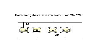
Number of Areas per ABR
ABRs will keep a copy of the database for all areas they service. If a router is connected to five areas for example, it will have to keep a list of five different databases. The number of areas per ABR is a number that is dependent on many factors, including type of area (normal, stub, NSSA), ABR CPU power, number of routes per area, and number of external routes per area. For this reason, a specific number of areas per ABR cannot be recommended. Of course, it's better not to overload an ABR when you can always spread the areas over other routers. The following diagram shows the difference between one ABR holding five different databases (including area 0) and two ABRs holding three databases each. Again, these are just guidelines, the more areas you configure per ABR the lower performance you get. In some cases, the lower performance can be tolerated.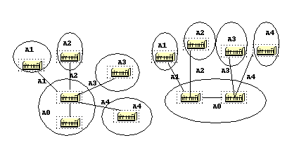
Full Mesh vs. Partial Mesh
Non Broadcast Multi-Access (NBMA) clouds such as Frame Relay or X.25, are always a challenge. The combination of low bandwidth and too many link-states is a recipe for problems. A partial mesh topology has proven to behave much better than a full mesh. A carefully laid out point-to-point or point-to-multipoint network works much better than multipoint networks that have to deal with DR issues.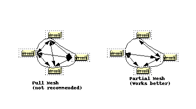
Memory Issues
It is not easy to figure out the memory needed for a particular OSPF configuration. Memory issues usually come up when too many external routes are injected in the OSPF domain. A backbone area with 40 routers and a default route to the outside world would have less memory issues compared with a backbone area with 4 routers and 33,000 external routes injected into OSPF.Memory could also be conserved by using a good OSPF design. Summarization at the area border routers and use of stub areas could further minimize the number of routes exchanged.
The total memory used by OSPF is the sum of the memory used in the routing table ( show ip route summary ) and the memory used in the link-state database. The following numbers are a rule of thumb estimate. Each entry in the routing table will consume between approximately 200 and 280 bytes plus 44 bytes per extra path. Each LSA will consume a 100 byte overhead plus the size of the actual link state advertisement, possibly another 60 to 100 bytes (for router links, this depends on the number of interfaces on the router). This should be added to memory used by other processes and by the IOS itself. If you really want to know the exact number, you can do a show memory with and without OSPF being turned on. The difference in the processor memory used would be the answer (keep a backup copy of the configs).
Normally, a routing table with less than 500K bytes could be accommodated with 2 to 4 MB RAM; Large networks with greater than 500K may need 8 to 16 MB, or 32 to 64 MB if full routes are injected from the Internet.
Summary
The OSPF protocol defined in RFC 1583, provides a high functionality open protocol that allows multiple vendor networks to communicate using the TCP/IP protocol family. Some of the benefits of OSPF are, fast convergence, VLSM, authentication, hierarchical segmentation, route summarization, and aggregation which are needed to handle large and complicated networks.Appendix A: Link-State Database Synchronization
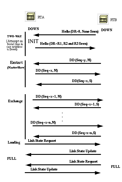
In the above diagram, routers on the same segment go through a series of states before forming a successful adjacency. The neighbor and DR election are done via the Hello protocol. Whenever a router sees itself in his neighbor's Hello packet, the state transitions to "2-Way". At that point DR and BDR election is performed on multi-access segments. A router continues forming an adjacency with a neighbor if either of the two routers is a DR or BDR or they are connected via a point-to-point or virtual link.
In the Exstart state,the two neighbors form a Master/Slave relationship where they agree on a initial sequence number. The sequence number is used to detect old or duplicate Link-State Advertisements (LSA).
In the Exchange state, Database Description Packets (DD) will get exchanged. These are abbreviated link-state advertisements in the form of link-state headers. The header supplies enough information to identify a link. The master node sends DD packets which are acknowledged with DD packets from the slave node. All adjacencies in exchange state or greater are used by the flooding procedure. These adjacencies are fully capable of transmitting and receiving all types of OSPF routing protocol packets.
In the Loading state, link-state request packets are sent to neighbors, asking for more recent advertisements that have been discovered but not yet received. Each router builds a list of required LSAs to bring its adjacency up to date. A Retransmission List is maintained to make sure that every LSA is acknowledged. To specify the number of seconds between link-state advertisement retransmissions for the adjacency you can use:
Link-state update packets are sent in response to request packets. The link-state update packets will be flooded over all adjacencies.ip ospf retransmit-interval seconds
In the Full state, the neighbor routers are fully adjacent. The databases for a common area are an exact match between adjacent routers.
Each LSA has an age field that gets periodically incremented while it is contained in the database or as it gets flooded throughout the area. When an LSA reaches a Maxage it gets flushed from the database if that LSA is not on any neighbors retransmission list.
Link-State Advertisements
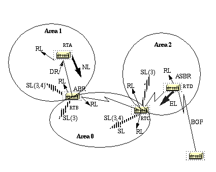
Link-state advertisements are broken into five types. Router Links (RL) are generated by all routers. These links describe the state of the router interfaces inside a particular area. These links are only flooded inside the router's area. Network Links (NL) are generated by a DR of a particular segment; these are an indication of the routers connected to that segment. Summary Links (SL) are the inter-area links (type 3); these links will list the networks inside other areas but still belonging to the autonomous system. Summary links are injected by the ABR from the backbone into other areas and from other areas into the backbone. These links are used for aggregation between areas. Other types of summary links are the asbr-summary links. These are type 4 links that point to the ASBR. This is to make sure that all routers know the way to exit the autonomous system. The last type is type 5, External Links (EL), these are injected by the ASBR into the domain.
The above diagram illustrates the different link types. RTA generates a router link (RL) into area 1, and it also generates a network link (NL) since it happens the be the DR on that particular segment. RTB is an ABR, and it generates RL into area 1 and area 0. RTB also generates summary links into area 1 and area 0. These links are the list of networks that are interchanged between the two areas. An ASBR summary link is also injected by RTB into area 1. This is an indication of the existence of RTD, the autonomous system boundary router (ASBR). Similarly RTC, which is another ABR, generates RL for area 0 and area 2, and a SL (3) into area 2 (since it is not announcing any ASBR), and a SL (3,4) into area 0 announcing RTD. RTD generates a RL for area 2 and generates an EL for external routes learned via BGP. The external routers will be flooded all over the domain.
The following table is a summary of the link state advertisements.
| LS Type | Advertisement Description |
|---|---|
| 1 | Router Link advertisements. Generated by each router for each area it belongs to. They describe the states of the router's link to the area. These are only flooded within a particular area. |
| 2 | Network Link advertisements. Generated by Designated Routers. They describe the set of routers attached to a particular network. Flooded in the area that contains the network. |
| 3 or 4 | Summary Link advertisements. Generated by Area Border routers. They describe inter-area (between areas) routes. Type 3 describes routes to networks, also used for aggregating routes. Type 4 describes routes to ASBR. |
| 5 | AS external link advertisements. Originated by ASBR. They describe routes to destinations external to the AS. Flooded all over except stub areas. |
The Link-State ID basically defines the identity of the link-state depending on the LS type. Router Links are identified by the router ID (RID) of the router that originated the advertisement. Network Links are identified by the relative IP address of the DR. This makes sense because Network Links are originated by the Designated Router. Summary Links (type 3) are identified by the IP network numbers of the destinations they are pointing at. ASBR Summary Links (Summary Links type 4) are identified by the RID of the ASBR. Finally, External Links are identified by the IP network numbers of the external destinations they are pointing at. The following table summarizes this information:
| LS Type | Link State ID (In the high level view of the database when referencing a router this is called Link ID) |
|---|---|
| 1 | The originating Router's Router ID (RID). |
| 2 | The IP interface address of the network's Designated Router. |
| 3 | The destination network number. |
| 4 | The router ID of the described AS boundary router. |
| 5 | The external network number. |
Stub network links: This term has nothing to do with stub areas. A stub segment is a segment that has one router only attached to it. An Ethernet or Token Ring segment that has one attached router is considered a link to a stub network. A loopback interface is also considered a link to stub network with a 255.255.255.255 mask (Host route).
Point-to-point links: These could be physical or logical (subinterfaces) point-to-point serial link connections. These links could be numbered (an IP address is configured on the link) or unnumbered.
Transit links: These are interfaces connected to networks that have more than one router attached, hence the name transit.
Virtual links: These are logical links that connect areas that do not have physical connections to the backbone. Virtual links are treated as numbered point-to-point links.
The link-ID is an identification of the link itself. This is different for each link type. A transit link is identified by the IP address of the DR on that link. A numbered point-to-point link is identified by the RID of the neighbor router on the point-to-point link. Virtual links are identical to point-to-point links. Finally, links to stub networks are identified by the IP address of the interface to the stub network. The following table summarizes this information:
| Link Type | Link ID (This applies to individual Links) |
|---|---|
| Point-to-Point | Neighbor Router ID |
| Link to transit network | Interface address of DR |
| Link to stub network (In case of loopback mask is 255.255.255.255) | Network/subnet number |
| Virtual Link | Neighbor Router ID |
| Link Type | Link Data |
|---|---|
| Stub network | Network Mask |
| Other networks (applies to router links only) | Router's associated IP interface address |
OSPF Database Example
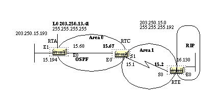
Given the network diagram above, the following configurations, and the IP route tables, let us look at different ways of understanding the OSPF database.
RTA#
 interface Loopback0
  ip address 203.250.13.41 255.255.255.255

 interface Ethernet0
  ip address 203.250.15.68 255.255.255.192

 interface Ethernet1
  ip address 203.250.15.193 255.255.255.192

 router ospf 10
  network 203.250.0.0 0.0.255.255 area 0

 RTA#show ip route
 Codes: C - connected, S - static, I - IGRP, R - RIP, M - mobile, B - BGP
        D - EIGRP, EX - EIGRP external, O - OSPF, IA - OSPF inter area
        E1 - OSPF external type 1, E2 - OSPF external type 2, E - EGP
        i - IS-IS, L1 - IS-IS level-1, L2 - IS-IS level-2, * - candidate default

 Gateway of last resort is 203.250.15.67 to network 0.0.0.0

      203.250.16.0 255.255.255.192 is subnetted, 1 subnets
 O E2    203.250.16.128 [110/10] via 203.250.15.67, 00:00:50, Ethernet0
      203.250.13.0 255.255.255.255 is subnetted, 1 subnets
 C       203.250.13.41 is directly connected, Loopback0
      203.250.15.0 255.255.255.192 is subnetted, 3 subnets
 O IA    203.250.15.0 [110/74] via 203.250.15.67, 00:00:50, Ethernet0
 C       203.250.15.64 is directly connected, Ethernet0
 C       203.250.15.192 is directly connected, Ethernet1
 O*E2 0.0.0.0 0.0.0.0 [110/10] via 203.250.15.67, 00:00:50, Ethernet0

 RTE#
 ip subnet-zero

 interface Ethernet0
  ip address 203.250.16.130 255.255.255.192

 interface Serial0
  ip address 203.250.15.2 255.255.255.192

 router ospf 10
  redistribute rip metric 10 subnets
  network 203.250.15.0 0.0.0.63 area 1
  default-information originate metric 10

 router rip
  network 203.250.16.0

 ip route 0.0.0.0 0.0.0.0 Ethernet0

RTE#show ip route
 Codes: C - connected, S - static, I - IGRP, R - RIP, M - mobile, B - BGP
        D - EIGRP, EX - EIGRP external, O - OSPF, IA - OSPF inter area
        E1 - OSPF external type 1, E2 - OSPF external type 2, E - EGP
        i - IS-IS, L1 - IS-IS level-1, L2 - IS-IS level-2, * - candidate default

 Gateway of last resort is 0.0.0.0 to network 0.0.0.0

      203.250.16.0 255.255.255.192 is subnetted, 1 subnets
 C       203.250.16.128 is directly connected, Ethernet0
      203.250.13.0 is variably subnetted, 2 subnets, 2 masks
 O IA    203.250.13.41 255.255.255.255
            [110/75] via 203.250.15.1, 00:16:31, Serial0
      203.250.15.0 255.255.255.192 is subnetted, 3 subnets
 C       203.250.15.0 is directly connected, Serial0
 O IA    203.250.15.64 [110/74] via 203.250.15.1, 00:16:31, Serial0
 O IA    203.250.15.192 [110/84] via 203.250.15.1, 00:16:31, Serial0
 S*   0.0.0.0 0.0.0.0 is directly connected, Ethernet0

 RTC#
 ip subnet-zero

 interface Ethernet0
  ip address 203.250.15.67 255.255.255.192

 interface Serial1
  ip address 203.250.15.1 255.255.255.192

 router ospf 10
  network 203.250.15.64 0.0.0.63 area 0
  network 203.250.15.0 0.0.0.63 area 1

RTF#show ip route
 Codes: C - connected, S - static, I - IGRP, R - RIP, M - mobile, B - BGP
        D - EIGRP, EX - EIGRP external, O - OSPF, IA - OSPF inter area
        E1 - OSPF external type 1, E2 - OSPF external type 2, E - EGP
        i - IS-IS, L1 - IS-IS level-1, L2 - IS-IS level-2, * - candidate default

 Gateway of last resort is 203.250.15.2 to network 0.0.0.0

      203.250.16.0 255.255.255.192 is subnetted, 1 subnets
 O E2    203.250.16.128 [110/10] via 203.250.15.2, 04:49:05, Serial1
      203.250.13.0 255.255.255.255 is subnetted, 1 subnets
 O       203.250.13.41 [110/11] via 203.250.15.68, 04:49:06, Ethernet0
      203.250.15.0 255.255.255.192 is subnetted, 3 subnets
 C       203.250.15.0 is directly connected, Serial1
 C       203.250.15.64 is directly connected, Ethernet0
 O       203.250.15.192 [110/20] via 203.250.15.68, 04:49:06, Ethernet0
 O*E2 0.0.0.0 0.0.0.0 [110/10] via 203.250.15.2, 04:49:06, Serial1
General View of the Database
RTC#show ip ospf database

       OSPF Router with ID (203.250.15.67) (Process ID 10)

                Router Link States (Area 1)

Link ID         ADV Router      Age    Seq#       Checksum Link count
203.250.15.67   203.250.15.67   48     0x80000008 0xB112   2
203.250.16.130  203.250.16.130  212    0x80000006 0x3F44   2

                Summary Net Link States (Area 1)

Link ID         ADV Router      Age    Seq#       Checksum
203.250.13.41   203.250.15.67   602    0x80000002 0x90AA
203.250.15.64   203.250.15.67   620    0x800000E9 0x3E3C
203.250.15.192  203.250.15.67   638    0x800000E5 0xA54E

                Router Link States (Area 0)

Link ID         ADV Router      Age    Seq#       Checksum Link count
203.250.13.41   203.250.13.41   179    0x80000029 0x9ADA   3
203.250.15.67   203.250.15.67   675    0x800001E2 0xDD23   1

                Net Link States (Area 0)

Link ID         ADV Router      Age    Seq#       Checksum
203.250.15.68   203.250.13.41   334    0x80000001 0xB6B5

                Summary Net Link States (Area 0)

Link ID         ADV Router      Age    Seq#       Checksum
203.250.15.0    203.250.15.67   792    0x80000002 0xAEBD

                Summary ASB Link States (Area 0)

Link ID         ADV Router      Age    Seq#       Checksum
203.250.16.130  203.250.15.67   579    0x80000001 0xF9AF

                AS External Link States

Link ID         ADV Router      Age    Seq#       Checksum Tag
0.0.0.0         203.250.16.130  1787   0x80000001 0x98CE   10
203.250.16.128  203.250.16.130  5      0x80000002 0x93C4   0
This is a general look at the whole OSPF database. The database is
listed according to the areas. In this case, we are looking at RTC's database
which is an ABR. Both area 1 and area 0's databases are listed. Area 1 is
composed of router links and summary links. No network links exist because no
DR exists on any of the segments in area 1. No Summary ASBR links exist in area
1 because the only ASBR happens to be in area 0. External links do not belong
to any particular area as they are flooded all over. Note that all the links
are the cumulative links collected from all routers in an area. We will mainly concentrate on the database in area 0. The Link-ID indicated here is actually the Link-State ID. This is a representation of the whole router, not a particular link. This is a bit confusing, but just remember that this high level Link-ID (should be Link-State ID) represents the whole router and not just a link.
Router Links
We will start with the router links. There are two entries listed for 203.250.13.41 and 203.250.15.67, these are the RIDs of the two routers in area 0. The number of links in area 0 for each router is also indicated. RTA has three links to area 0 and RTC has one link. A detailed view of RTC's router links follows:Router Link States (Area 0) Link ID ADV Router Age Seq# Checksum Link count 203.250.13.41 203.250.13.41 179 0x80000029 0x9ADA 3 203.250.15.67 203.250.15.67 675 0x800001E2 0xDD23 1
RTC#show ip ospf database router 203.250.15.67

     OSPF Router with ID (203.250.15.67) (Process ID 10)

                Router Link States (Area 1)

  LS age: 1169
  Options: (No TOS-capability)
  LS Type: Router Links
  Link State ID: 203.250.15.67
  Advertising Router: 203.250.15.67
  LS Seq Number: 80000008
  Checksum: 0xB112
  Length: 48
  Area Border Router
   Number of Links: 2

    Link connected to: another Router (point-to-point)
     (Link ID) Neighboring Router ID: 203.250.16.130
     (Link Data) Router Interface address: 203.250.15.1
      Number of TOS metrics: 0
       TOS 0 Metrics: 64

    Link connected to: a Stub Network
     (Link ID) Network/subnet number: 203.250.15.0
     (Link Data) Network Mask: 255.255.255.192
      Number of TOS metrics: 0
       TOS 0 Metrics: 64
One thing to note here is that OSPF generates an extra stub link for
each point-to-point interface. Do not get confused if you see the link count
larger than the number of physical interfaces.
Router Link States (Area 0)

  LS age: 1227
  Options: (No TOS-capability)
  LS Type: Router Links
  Link State ID: 203.250.15.67
  Advertising Router: 203.250.15.67
  LS Seq Number: 80000003
  Checksum: 0xA041
  Length: 36
  Area Border Router
   Number of Links: 1

    Link connected to: a Transit Network
     (Link ID) Designated Router address: 203.250.15.68
     (Link Data) Router Interface address: 203.250.15.67
      Number of TOS metrics: 0
       TOS 0 Metrics: 10
Note that the Link ID is equal to the IP address (not the RID) of the
attached DR; in this case it is 203.250.15.68. The Link Data is RTC's own IP
address. Network Links
One network link is listed, indicated by the interface IP address (not the RID) of the DR, in this case 203.250.15.68. A detailed view of this entry follows:Net Link States (Area 0) Link ID ADV Router Age Seq# Checksum 203.250.15.68 203.250.13.41 334 0x80000001 0xB6B5
RTC#show ip ospf database network

       OSPF Router with ID (203.250.15.67) (Process ID 10)

                Net Link States (Area 0)

  Routing Bit Set on this LSA
  LS age: 1549
  Options: (No TOS-capability)
  LS Type: Network Links
  Link State ID: 203.250.15.68 (address of Designated Router)
  Advertising Router: 203.250.13.41
  LS Seq Number: 80000002
  Checksum: 0xB4B6
  Length: 32
  Network Mask: 255.255.255.192

        Attached Router: 203.250.13.41
        Attached Router: 203.250.15.67
Note that the network link lists the RIDs of the routers attached to
the transit network; in this case the RIDs of RTA and RTC are listed. Summary Links
Summary Net Link States (Area 0)

Link ID         ADV Router      Age    Seq#       Checksum
203.250.15.0    203.250.15.67   792    0x80000002 0xAEBD
Area 0 has one summary link represented by the IP network address of the
link 203.250.15.0. This link was injected by the ABR RTC from area 1 into
area 0. A detailed view of this summary link follows, summary links for
area 1 are not listed here:

RTC#show ip ospf database summary (area 1 is not listed)

              Summary Net Link States (Area 0)

  LS age: 615
  Options: (No TOS-capability)
  LS Type: Summary Links(Network)
  Link State ID: 203.250.15.0 (summary Network Number)
  Advertising Router: 203.250.15.67
  LS Seq Number: 80000003
  Checksum: 0xACBE
  Length: 28
  Network Mask: 255.255.255.192 TOS: 0  Metric: 64
Summary ASBR Links This is an indication of who the ASBR is. In this case the ASBR is RTE represented by its RID 203.250.16.130. The advertising router for this entry into area 0 is RTC with RID 203.250.15.67. A detailed view of the summary ASBR entry follows:Summary ASB Link States (Area 0) Link ID ADV Router Age Seq# Checksum 203.250.16.130 203.250.15.67 579 0x80000001 0xF9AF
RTC#show ip ospf database asbr-summary

        OSPF Router with ID (203.250.15.67) (Process ID 10)

                 Summary ASB Link States (Area 0)

   LS age: 802
   Options: (No TOS-capability)
   LS Type: Summary Links(AS Boundary Router)
   Link State ID: 203.250.16.130 (AS Boundary Router address)
   Advertising Router: 203.250.15.67
   LS Seq Number: 80000003
   Checksum: 0xF5B1
   Length: 28
   Network Mask: 0.0.0.0 TOS: 0  Metric: 64
External Links We have two external Links, the first one is the 0.0.0.0 injected into OSPF via the default-information originate command. The other entry is network 203.250.16.12 8 which is injected into OSPF by redistribution. The router advertising these networks is 203.250.16.130, the RID of RTE. The following is the detailed view of the external routes:AS External Link States Link ID ADV Router Age Seq# Checksum Tag 0.0.0.0 203.250.16.130 1787 0x80000001 0x98CE 10 203.250.16.128 203.250.16.130 5 0x80000002 0x93C4 0
RTC#show ip ospf database external

        OSPF Router with ID (203.250.15.67) (Process ID 10)

                 AS External Link States

   Routing Bit Set on this LSA
   LS age: 208
   Options: (No TOS-capability)
   LS Type: AS External Link
   Link State ID: 0.0.0.0 (External Network Number )
   Advertising Router: 203.250.16.130
   LS Seq Number: 80000002
   Checksum: 0x96CF
   Length: 36
   Network Mask: 0.0.0.0
         Metric Type: 2 (Larger than any link state path)
         TOS: 0
         Metric: 10
         Forward Address: 0.0.0.0
         External Route Tag: 10

  Routing Bit Set on this LSA
   LS age: 226
   Options: (No TOS-capability)
   LS Type: AS External Link
   Link State ID: 203.250.16.128 (External Network Number)
   Advertising Router: 203.250.16.130
   LS Seq Number: 80000002
   Checksum: 0x93C4
   Length: 36
   Network Mask: 255.255.255.192
         Metric Type: 2 (Larger than any link state path)
         TOS: 0
         Metric: 10
         Forward Address: 0.0.0.0
         External Route Tag: 0
Note the forward address. Whenever this address is 0.0.0.0 it indicates
that the external routes are reachable via the advertising router, in this case
203. 250.16.130. This is why the identity of the ASBR is injected by ABRs into
other areas using ASBR summary links. This forward address is not always 0.0.0.0. In some cases, it could be the IP address of another router on the same segment. The following diagram will illustrate this situation:
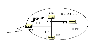
In the above situation RTB, is running BGP with RTA, and OSPF with the rest of the domain. RTA is not running OSPF. RTB is redistributing BGP routes into OSPF. According to OSPF, RTB is an ASBR advertising external routes. The forwarding address in this case is set to 125.211.1.1 and not to the advertising router (0.0.0.0) RT B. This makes sense because there is no need to make the extra hop. An important thing to remember is that routers inside the OSPF domain should be able to reach the forwarding address via OSPF in order for the external routes to be put in the IP routing table. If the forwarding address is reached via some other protocol or no t accessible, the external entries would be in the database but not in the IP routing table.
Another situation would arise if both RTB and RTC are ASBRs (RTC is also running BGP with RTA). In this situation, in order to eliminate the duplication of the effort, one of the two routers will not advertise (will flush) the external routes. T he router with the higher RID will win.
The Full Database
Finally, this is a listing of the whole database as an exercise. You should now b e able to go over each entry and explain what is going on:
RTC#show ip ospf database router

         OSPF Router with ID (203.250.15.67) (Process ID 10)

                 Router Link States (Area 1)

   LS age: 926
   Options: (No TOS-capability)
   LS Type: Router Links
   Link State ID: 203.250.15.67
   Advertising Router: 203.250.15.67
   LS Seq Number: 80000035
   Checksum: 0x573F
   Length: 48
   Area Border Router
    Number of Links: 2
     Link connected to: another Router (point-to-point)
      (Link ID) Neighboring Router ID: 203.250.16.130
      (Link Data) Router Interface address: 203.250.15.1
       Number of TOS metrics: 0
        TOS 0 Metrics: 64

     Link connected to: a Stub Network
      (Link ID) Network/subnet number: 203.250.15.0
      (Link Data) Network Mask: 255.255.255.192
       Number of TOS metrics: 0
        TOS 0 Metrics: 64

   Routing Bit Set on this LSA
   LS age: 958
   Options: (No TOS-capability)
   LS Type: Router Links
   Link State ID: 203.250.16.130
   Advertising Router: 203.250.16.130
   LS Seq Number: 80000038
   Checksum: 0xDA76
   Length: 48
   AS Boundary Router
    Number of Links: 2

     Link connected to: another Router (point-to-point)
      (Link ID) Neighboring Router ID: 203.250.15.67
      (Link Data) Router Interface address: 203.250.15.2
       Number of TOS metrics: 0
        TOS 0 Metrics: 64

     Link connected to: a Stub Network
      (Link ID) Network/subnet number: 203.250.15.0
      (Link Data) Network Mask: 255.255.255.192
       Number of TOS metrics: 0
        TOS 0 Metrics: 64

                 Router Link States (Area 0)

   Routing Bit Set on this LSA
   LS age: 1107
   Options: (No TOS-capability)
   LS Type: Router Links
   Link State ID: 203.250.13.41
   Advertising Router: 203.250.13.41
   LS Seq Number: 8000002A
   Checksum: 0xC0B0
   Length: 60
   AS Boundary Router
    Number of Links: 3

     Link connected to: a Stub Network
      (Link ID) Network/subnet number: 203.250.13.41
      (Link Data) Network Mask: 255.255.255.255
       Number of TOS metrics: 0
        TOS 0 Metrics: 1

     Link connected to: a Stub Network
      (Link ID) Network/subnet number: 203.250.15.192
      (Link Data) Network Mask: 255.255.255.192
       Number of TOS metrics: 0
        TOS 0 Metrics: 10

     Link connected to: a Transit Network
      (Link ID) Designated Router address: 203.250.15.68
      (Link Data) Router Interface address: 203.250.15.68
       Number of TOS metrics: 0
        TOS 0 Metrics: 10

   LS age: 1575
   Options: (No TOS-capability)
   LS Type: Router Links
   Link State ID: 203.250.15.67
   Advertising Router: 203.250.15.67
   LS Seq Number: 80000028
   Checksum: 0x5666
   Length: 36
   Area Border Router
    Number of Links: 1

     Link connected to: a Transit Network
      (Link ID) Designated Router address: 203.250.15.68
      (Link Data) Router Interface address: 203.250.15.67
       Number of TOS metrics: 0
        TOS 0 Metrics: 10

 RTC#show ip ospf database network

        OSPF Router with ID (203.250.15.67) (Process ID 10)

                 Net Link States (Area 0)

   Routing Bit Set on this LSA
   LS age: 1725
   Options: (No TOS-capability)
   LS Type: Network Links
   Link State ID: 203.250.15.68 (address of Designated Router)
   Advertising Router: 203.250.13.41
   LS Seq Number: 80000026
   Checksum: 0x6CDA
   Length: 32
   Network Mask: 255.255.255.192
         Attached Router: 203.250.13.41
         Attached Router: 203.250.15.67

 RTC#show ip ospf database summary

        OSPF Router with ID (203.250.15.67) (Process ID 10)

                 Summary Net Link States (Area 1)

   LS age: 8
   Options: (No TOS-capability)
   LS Type: Summary Links(Network)
   Link State ID: 203.250.13.41 (summary Network Number)
   Advertising Router: 203.250.15.67
   LS Seq Number: 80000029
   Checksum: 0x42D1
   Length: 28
   Network Mask: 255.255.255.255 TOS: 0  Metric: 11

   LS age: 26
   Options: (No TOS-capability)
   LS Type: Summary Links(Network)
   Link State ID: 203.250.15.64 (summary Network Number)
   Advertising Router: 203.250.15.67
   LS Seq Number: 80000030
   Checksum: 0xB182
   Length: 28
   Network Mask: 255.255.255.192 TOS: 0  Metric: 10

   LS age: 47
   Options: (No TOS-capability)
   LS Type: Summary Links(Network)
   Link State ID: 203.250.15.192 (summary Network Number)
   Advertising Router: 203.250.15.67
   LS Seq Number: 80000029
   Checksum: 0x1F91
   Length: 28
   Network Mask: 255.255.255.192 TOS: 0  Metric: 20

                 Summary Net Link States (Area 0)

   LS age: 66
   Options: (No TOS-capability)
   LS Type: Summary Links(Network)
   Link State ID: 203.250.15.0 (summary Network Number)
   Advertising Router: 203.250.15.67
   LS Seq Number: 80000025
   Checksum: 0x68E0
   Length: 28
   Network Mask: 255.255.255.192 TOS: 0  Metric: 64

 RTC#show ip ospf asbr-summary

        OSPF Router with ID (203.250.15.67) (Process ID 10)

                 Summary ASB Link States (Area 0)

   LS age: 576
   Options: (No TOS-capability)
   LS Type: Summary Links(AS Boundary Router)
   Link State ID: 203.250.16.130 (AS Boundary Router address)
   Advertising Router: 203.250.15.67
   LS Seq Number: 80000024
   Checksum: 0xB3D2
   Length: 28
   Network Mask: 0.0.0.0 TOS: 0  Metric: 64


 RTC#show ip ospf database external

       OSPF Router with ID (203.250.15.67) (Process ID 10)

                 AS External Link States

   Routing Bit Set on this LSA
   LS age: 305
   Options: (No TOS-capability)
   LS Type: AS External Link
   Link State ID: 0.0.0.0 (External Network Number)
   Advertising Router: 203.250.16.130
   LS Seq Number: 80000001
   Checksum: 0x98CE
   Length: 36
   Network Mask: 0.0.0.0
         Metric Type: 2 (Larger than any link state path)
         TOS: 0
         Metric: 10
         Forward Address: 0.0.0.0
         External Route Tag: 10

   Routing Bit Set on this LSA
   LS age: 653
   Options: (No TOS-capability)
   LS Type: AS External Link
   Link State ID: 203.250.16.128 (External Network Number)
   Advertising Router: 203.250.16.130
   LS Seq Number: 80000024
   Checksum: 0x4FE6
   Length: 36
   Network Mask: 255.255.255.192
         Metric Type: 2 (Larger than any link state path)
         TOS: 0
         Metric: 10
         Forward Address: 0.0.0.0
         External Route Tag: 0
Appendix B: OSPF and IP Multicast Addressing
OSPF used IP multicast to exchange Hello packets and Link State Updates. An IP multicast address is implemented using class D addresses. A class D address ranges from 224.0.0.0 to 239.255.255.255.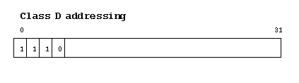
Some special IP multicast addresses are reserved for OSPF:
-
224.0.0.5: All OSPF routers should be able to transmit and listen to
this address.
-
224.0.0.6: All DR and BDR routers should be able to transmit and
listen to this address.
For multiaccess networks that support multicast, the low order 23 bits of the IP address are used as the low order bits of the MAC multicast address 01-005E-00-00- 00. For example:
-
224.0.0.5 would be mapped to 01-00-5E-00-00-05
-
224.0.0.6 would be mapped to
01-00-5E-00-00-06
Appendix C: Variable Length Subnet Masks (VLSM)
The following is a binary/decimal conversion chart:| 0000 | 0001 | 0010 | 0011 | 0100 | 0101 | 0110 | 0111 | ||||||||
|---|---|---|---|---|---|---|---|---|---|---|---|---|---|---|---|
| 0 | 0000 | 16 | 0000 | 32 | 0000 | 48 | 0000 | 64 | 0000 | 80 | 0000 | 96 | 0000 | 112 | 0000 |
| 1 | 0001 | 17 | 0001 | 33 | 0001 | 49 | 0001 | 65 | 0001 | 81 | 0001 | 97 | 0001 | 113 | 0001 |
| 2 | 0010 | 18 | 0010 | 34 | 0010 | 50 | 0010 | 66 | 0010 | 82 | 0010 | 98 | 0010 | 114 | 0010 |
| 3 | 0011 | 19 | 0011 | 35 | 0011 | 51 | 0011 | 67 | 0011 | 83 | 0011 | 99 | 0011 | 115 | 0011 |
| 4 | 0100 | 20 | 0100 | 36 | 0100 | 52 | 0100 | 68 | 0100 | 84 | 0100 | 100 | 0100 | 116 | 0100 |
| 5 | 0101 | 21 | 0101 | 37 | 0101 | 53 | 0101 | 69 | 0101 | 85 | 0101 | 101 | 0101 | 117 | 0101 |
| 6 | 0110 | 22 | 0110 | 38 | 0110 | 54 | 0110 | 70 | 0110 | 86 | 0110 | 102 | 0110 | 118 | 0110 |
| 7 | 0111 | 23 | 0111 | 39 | 0111 | 55 | 0111 | 71 | 0111 | 87 | 0111 | 103 | 0111 | 119 | 0111 |
| 8 | 1000 | 24 | 1000 | 40 | 1000 | 56 | 1000 | 72 | 1000 | 88 | 1000 | 104 | 1000 | 120 | 1000 |
| 9 | 1001 | 25 | 1001 | 41 | 1001 | 57 | 1001 | 73 | 1001 | 89 | 1001 | 105 | 1001 | 121 | 1001 |
| 10 | 1010 | 26 | 1010 | 42 | 1010 | 58 | 1010 | 74 | 1010 | 90 | 1010 | 106 | 1010 | 122 | 1010 |
| 11 | 1011 | 27 | 1011 | 43 | 1011 | 59 | 1011 | 75 | 1011 | 91 | 1011 | 107 | 1011 | 123 | 1011 |
| 12 | 1100 | 28 | 1100 | 44 | 1100 | 60 | 1100 | 76 | 1100 | 92 | 1100 | 108 | 1100 | 124 | 1100 |
| 13 | 1101 | 29 | 1101 | 45 | 1101 | 61 | 1101 | 77 | 1101 | 93 | 1101 | 109 | 1101 | 125 | 1101 |
| 14 | 1110 | 30 | 1110 | 46 | 1110 | 62 | 1110 | 78 | 1110 | 94 | 1110 | 110 | 1110 | 126 | 1110 |
| 15 | 1111 | 31 | 1111 | 47 | 1111 | 63 | 1111 | 79 | 1111 | 95 | 1111 | 111 | 1111 | 127 | 1111 |
| 1000 | 1001 | 1010 | 1011 | 1100 | 1101 | 1110 | 1111 | ||||||||
| 128 | 0000 | 144 | 0000 | 160 | 0000 | 176 | 0000 | 192 | 0000 | 208 | 0000 | 224 | 0000 | 240 | 0000 |
| 129 | 0001 | 145 | 0001 | 161 | 0001 | 177 | 0001 | 193 | 0001 | 209 | 0001 | 225 | 0001 | 241 | 0001 |
| 130 | 0010 | 146 | 0010 | 162 | 0010 | 178 | 0010 | 194 | 0010 | 210 | 0010 | 226 | 0010 | 242 | 0010 |
| 131 | 0011 | 147 | 0011 | 163 | 0011 | 179 | 0011 | 195 | 0011 | 211 | 0011 | 227 | 0011 | 243 | 0011 |
| 132 | 0100 | 148 | 0100 | 164 | 0100 | 180 | 0100 | 196 | 0100 | 212 | 0100 | 228 | 0100 | 244 | 0100 |
| 133 | 0101 | 149 | 0101 | 165 | 0101 | 181 | 0101 | 197 | 0101 | 213 | 0101 | 229 | 0101 | 245 | 0101 |
| 134 | 0110 | 150 | 0110 | 166 | 0110 | 182 | 0110 | 198 | 0110 | 214 | 0110 | 230 | 0110 | 246 | 0110 |
| 135 | 0111 | 151 | 0111 | 167 | 0111 | 183 | 0111 | 199 | 0111 | 215 | 0111 | 231 | 0111 | 247 | 0111 |
| 136 | 1000 | 152 | 1000 | 168 | 1000 | 184 | 1000 | 200 | 1000 | 216 | 1000 | 232 | 1000 | 248 | 1000 |
| 137 | 1001 | 153 | 1001 | 169 | 1001 | 185 | 1001 | 201 | 1001 | 217 | 1001 | 233 | 1001 | 249 | 1001 |
| 138 | 1010 | 154 | 1010 | 170 | 1010 | 186 | 1010 | 202 | 1010 | 218 | 1010 | 234 | 1010 | 250 | 1010 |
| 139 | 1011 | 155 | 1011 | 171 | 1011 | 187 | 1011 | 203 | 1011 | 219 | 1011 | 235 | 1011 | 251 | 1011 |
| 140 | 1100 | 156 | 1100 | 172 | 1100 | 188 | 1100 | 204 | 1100 | 220 | 1100 | 236 | 1100 | 252 | 1100 |
| 141 | 1101 | 157 | 1101 | 173 | 1101 | 189 | 1101 | 205 | 1101 | 221 | 1101 | 237 | 1101 | 253 | 1101 |
| 142 | 1110 | 158 | 1110 | 174 | 1110 | 190 | 1110 | 206 | 1110 | 222 | 1110 | 238 | 1110 | 254 | 1110 |
| 143 | 1111 | 159 | 1111 | 175 | 1111 | 191 | 1111 | 207 | 1111 | 223 | 1111 | 239 | 1111 | 255 | 1111 |
For example, suppose you were assigned a class C network 192.214.11.0 and you need to divide that network into three subnets with 100 hosts in one subnet and 50 hosts for each of the remaining subnets. Ignore the two end limits 0 and 255, and you have theoretically available to you 256 addresses (192.214.11.0 - 192.214.11.255). This cannot be done without VLSM.
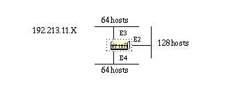
There are a handful of subnet masks that can be used; note that a mask should have a contiguous number of ones that start from the left and the rest of the bits are all 0s.
Without VLSM you have the choice to use mask 255.255.255.128 and divide the addresses into 2 subnets with 128 hosts each or use 255.255.255.192 and divide the space into 4 subnets with 64 hosts each. This does not meet the requirement. If you use multiple masks, you can use mask 128 and further subnet the second chunk of addresses with mask 192. This table shows how you have divided the address space accordingly.-252 (1111 1100) The address space is divided into 64. -248 (1111 1000) The address space is divided into 32. -240 (1111 0000) The address space is divided into 16. -224 (1110 0000) The address space is divided into 8. -192 (1100 0000) The address space is divided into 4. -128 (1000 0000) The address space is divided into 2.
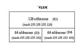
Now, be careful in allocating the IP addresses to each mask. Once you assign an IP address to the router or to a host, you have used up the whole subnet for that segment. For example, if you assign 192.214.11.10 255.255.255.128 to E2, the whole range of addresses between 192.214.11.0 and 192.214.11.127 is consumed by E2. In the same way if you assign 192.214.11.160 255.255.255.128 to E2, the whole range of addresses between 192.214.11.128 and 192.214.11.255 is consumed by the E2 segment.
This is an illustration of how the router interprets these addresses. Remember that any time you use a mask different than the natural mask, for instance if you are subnetting, the router complains if the combination IP address and mask result in a subnet zero. Use the ip subnet-zero command on the router in order to resolve this issue.
RTA#
 ip subnet-zero
 interface Ethernet2
  ip address 192.214.11.10 255.255.255.128
 interface Ethernet3
  ip address 192.214.11.160 255.255.255.192
 interface Ethernet4
  ip address 192.214.11.226 255.255.255.192

 RTA#show ip route connected
      192.214.11.0 is variably subnetted, 3 subnets, 2 masks
 C       192.214.11.0 255.255.255.128 is directly connected, Ethernet2
 C       192.214.11.128 255.255.255.192 is directly connected, Ethernet3
 C       192.214.11.192 255.255.255.192 is directly connected, Ethernet4
Nessun commento:
Posta un commento